Week 3 - External flow simulation over an Ahmed body.

AIM:

As the body is perfectly symmetric, we can simulate it by considering only half the body. This is the best practice where you can save on the number of cells and get the results faster as well.

The geometry that is provided with the challenge needs a modification which you should be able to do at this stage of a course. You need to use the 'split body' command in SpaceClaim to operate and then you can use the symmetry boundary condition in Fluent to perform the simulation.

Simulate the velocity of 25 m/sec with the default air properties in fluent.

For this challenge, you will have to provide answers to the following questions:

Q1. Describe Ahmed's body and its importance.

Q2. Explain the reason for the negative pressure in the wake region.

Q3. Explain the significance of the point of separation.

Expected Results:

1. Velocity and pressure contours.

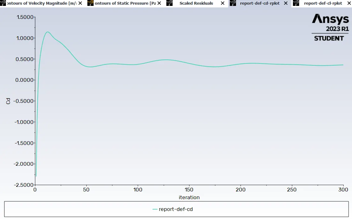
2. The drag coefficient plot for a refined case. (For a velocity of 25m/sec, the drag coefficient should be around 0.33).

3. The vector plot clearly shows the wake region.

4. Perform the grid independence test and provide the values of drag and lift with each case.

INTRODUCTION:

Ahmed's body is the 3D model that is representative of a standard passenger car. now, the reason this model was developed is to help invalidate a CFD code. so, To validate or trust your CFD code, we need to make sure that you know it gives you results that are comparable with say experimental data and that is where the Ahmed body comes in this is a research model which you know built in real life and people did an experimental analysis on it and then they have a lot of rich data and this date is available in the publication.

THEORY:

Mach number:

The Mach number is the dominant parameter in the compressible flow analysis, with different effects depending on its magnitude. Aerodynamicists especially make the distinction between the various ranges of Mach number and the following rough classification is commonly used:

1. Ma<0.3: incompressible flow - where the density effects are negligible.
2. 0.3<Ma<0.8: subsonic flow - Where the density effects are appear.
3. 0.8<Ma<1.2: transonic flow - where the shock wave first appears dividing the subsonic and supersonic region of the flow. Powered flight in the transonic region is difficult because of the mixed character of the field.
4. 1.2<Ma<3.0: supersonic flow - where shock waves are present but no subsonic regions.
5. 3.0

Density Based solver:

The density-based solver was developed for high-pressure compressible flow. It solves energy and momentum and continuity and species transport equations simultaneously. This solver is suitable for a supersonic solver. This solver is only for when the Mach number is greater than 0.3. There are two methods available in this Density-based solver. They are,

• Implicit.
• Explicit.

1. Implicit method:

In this method, the unknown values for each cell are solved by using existing values and unknown values from the neighboring cells. In this method, the equation is solved simultaneously. This method doesn't have strict limits on CFL constraints. The default courant number is 5. This method is highly suitable for hypersonic flow and shock interactions.

2. Explicit method:

In this method, the unknown values for each cell are solved by using existing values. Here the equations for unknown values in each cell are solved one at a time. In this method, the equation is not solved simultaneously. This method has strict limits on CFL constraints. In this method, the maximum limit on the courant number is 2. This method is highly suitable for the flow having a higher Mach number.

Reynolds Number:

The Reynolds number (Re) is dimensionless. It is defined as the ratio of inertial force to viscous force.

FORMULA, Re = (V*D)/nu

were, v = velocity of the fluid(m/s).

D = diameter of the fluid(m/s).

nu = kinematic viscosity of the fluid (m²/s).

Reynolds number is used in force convection. The force convection is a type of heat transfer, in which fluids are forced to move to increase the heat transfer. Reynolds number is used to predict the flow patterns in different fluid flow situations. At a low Reynolds number the flow tends to be Laminar flow, while at a high Reynolds number, the flow tends to be Turbulence flow.

• Re<2000, flow is Laminar for pipe.
• 2000<Re, flow is transition.
• Re>4000, flow is Turbulence for pipe.

K-Omega SST:

This model is essentially used for a low Reynolds number. this model takes "elliptic" near-wall behavior meaning that it has an inherent nature of being able to "communicate" with the wall and has Dirichlet (as in no-slip in this case) boundary conditions. the implication of such behavior is the straightforward possibility of integrating through the laminar sublayer without additional numerically destabilizing damping function or two additional transport equations.

1. First the initial layer thickness is calculated using the y+ formula, we can generate the mesh and set up the case for the first few iterations.
2. once we simulate the first few iterations, it is desirable to check the y+ value using the post-processing tool.
3. the flow physics can change over the surface so, checking and adjusting the first layer thickness in the initial stage of the simulation is important to avoid the re-meshing and wastage of computational resources.

Y Plus:

The concept of y+ is tied to the boundary layer theory. when the fluid flows over a wall, it tries to stick to the wall. this phenomenon is called the no-slip condition. during this condition, the subsequent layer of the fluid above the one that gets stuck to the wall will have a hindrance in their motion. this causes a sharp change in the properties of the fluid as one travels away from the wall.

Co-efficient of Drag:

Drag is caused due to the pressure difference between the frontal and rear end of the vehicle. the drag can be reduced by modification of the design of the vehicle or the modification of the airflow around the vehicle so that we can save energy up to 50% by modifying the drag coefficient.

PROCEDURE:

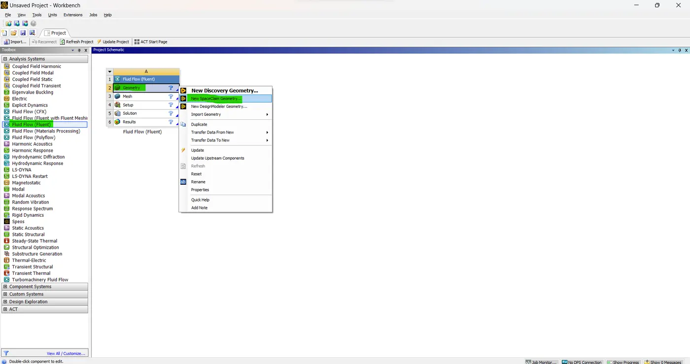
• the Ahmed body is a 3D model representative of a standard passenger car. Now the reason why this model was developed is to help invalidate CFD code.
• so, now open the ansys fluent -> create fluent -> open the geomentry -> and drag and drop the model.
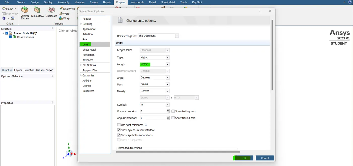
• The unit is in millimeters. so, we need to change the units to meters. so, goto files-> spaceclame option -> units -> change to meterv-> click "OK".
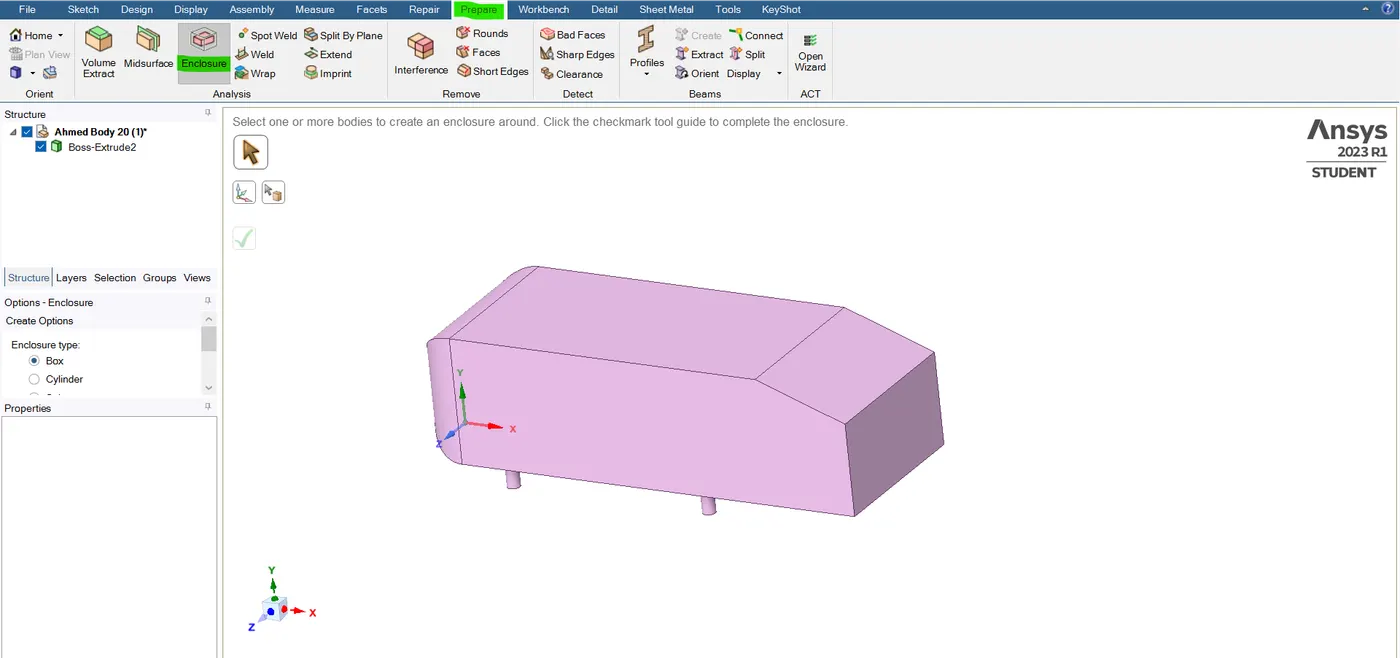
• No the modeling strategy is very simple, we want the flow to be simulated outside Ahmed's body, right? In other words, that is where the mesh needs to be created and you don't want the mesh to be inside Ahmed's body.

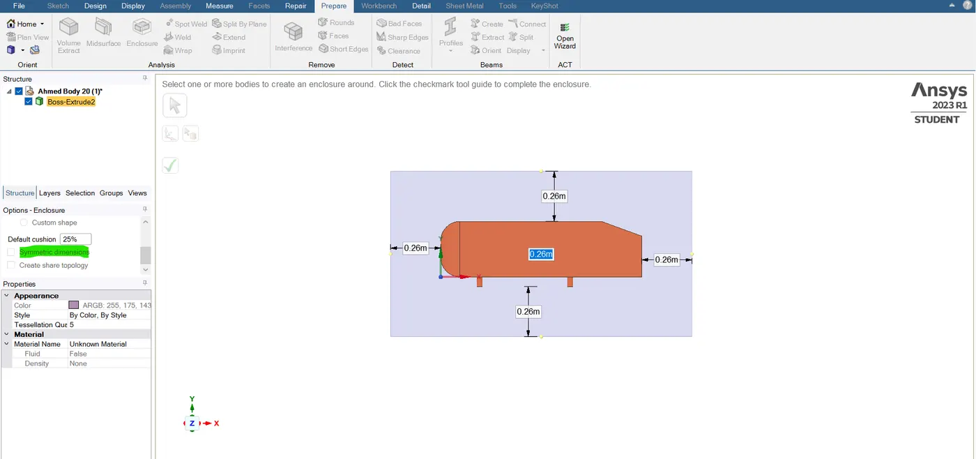
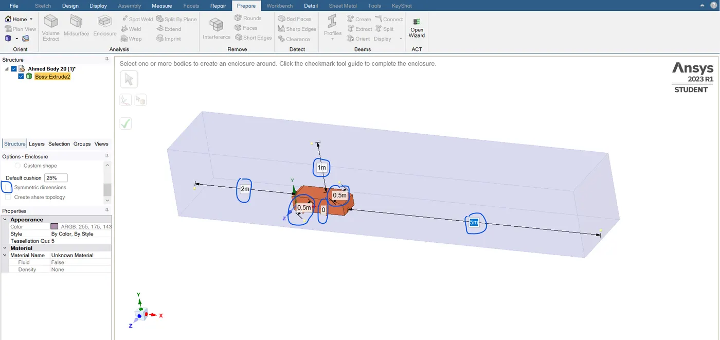
• the front of Ahmed's body is 5 meters and the back side of Ahmed's body is 2 meters. the bottom side is 0. and the top of Ahmed's body is 1 meter. and we adjusted the width parameter for which I'm going to be looking at the model's long y-axis is 0.5 and the x-axis is 0.5 meters and then click ok. but before doing this we need to uncheck the symmetry dimension.
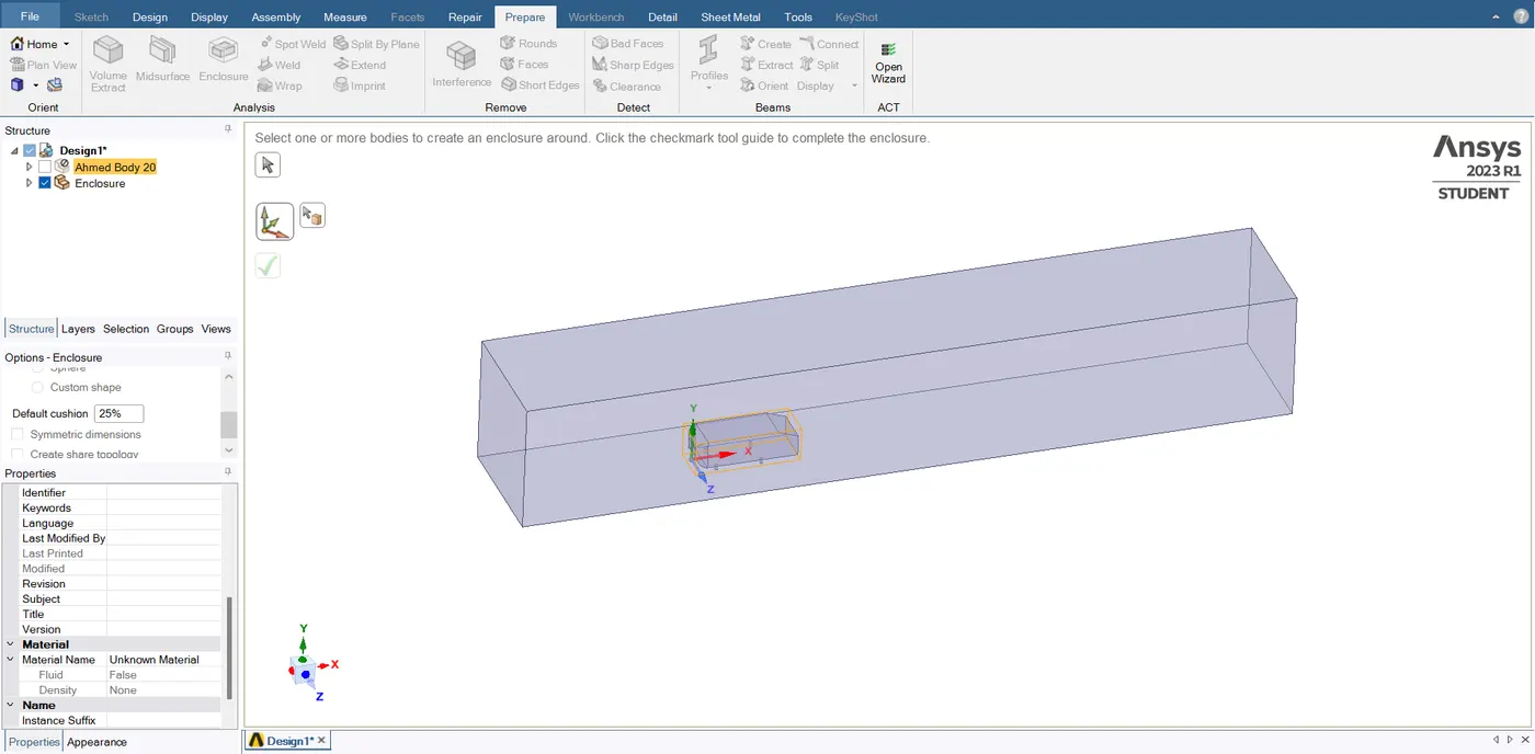
• so, now we just created the encloser we have two components. so the first one is the Ahmed body, which we imported originally. and secondly, we just added an encloser.
• so, the enclosure means it still looks like a box that contains Ahmed's body. yes, but the key difference is that space claims are automatically created.

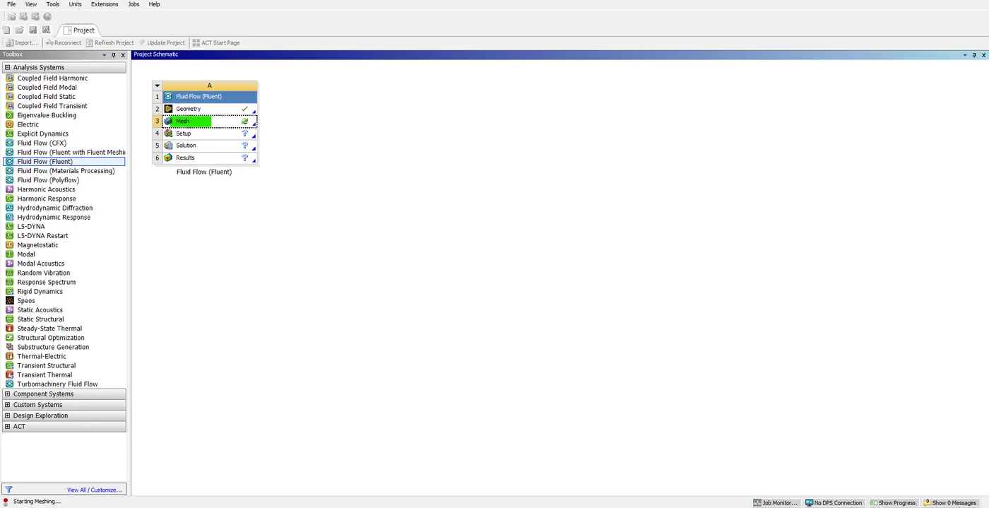
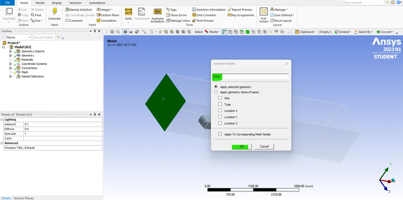
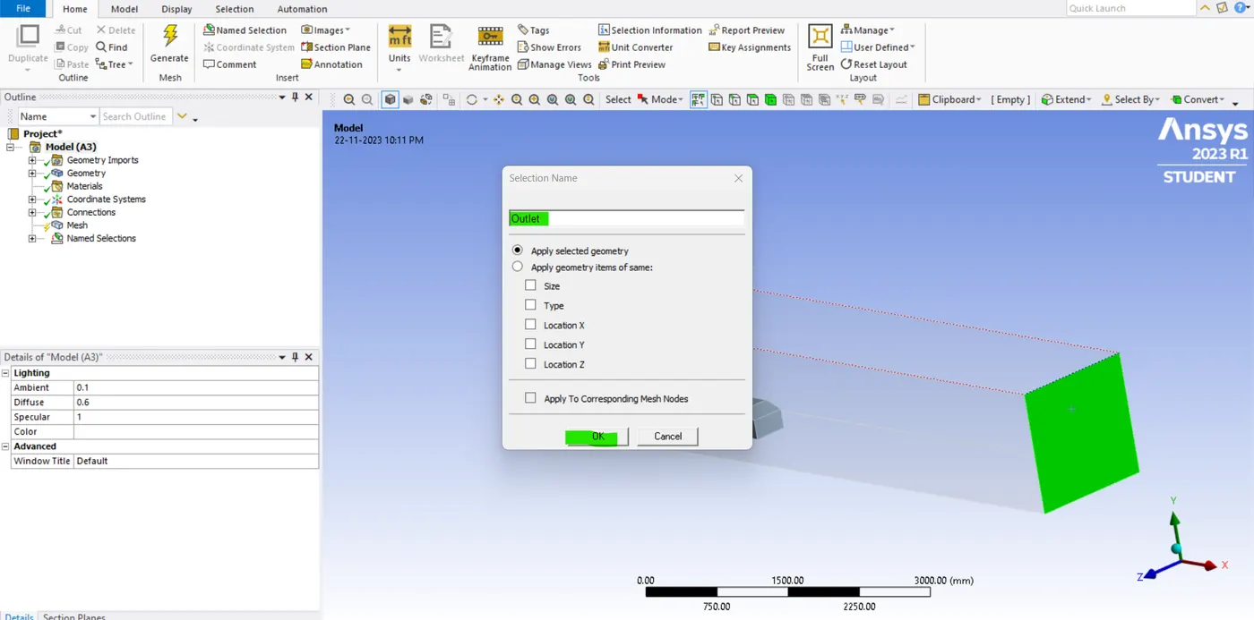
• now just select the plain option and select the "selection mode" Now we can see that Ahmed's body is automatically been cut and this is exactly what we need for the simulation. now just close this GUI or geomentry and open the mesh GUI.
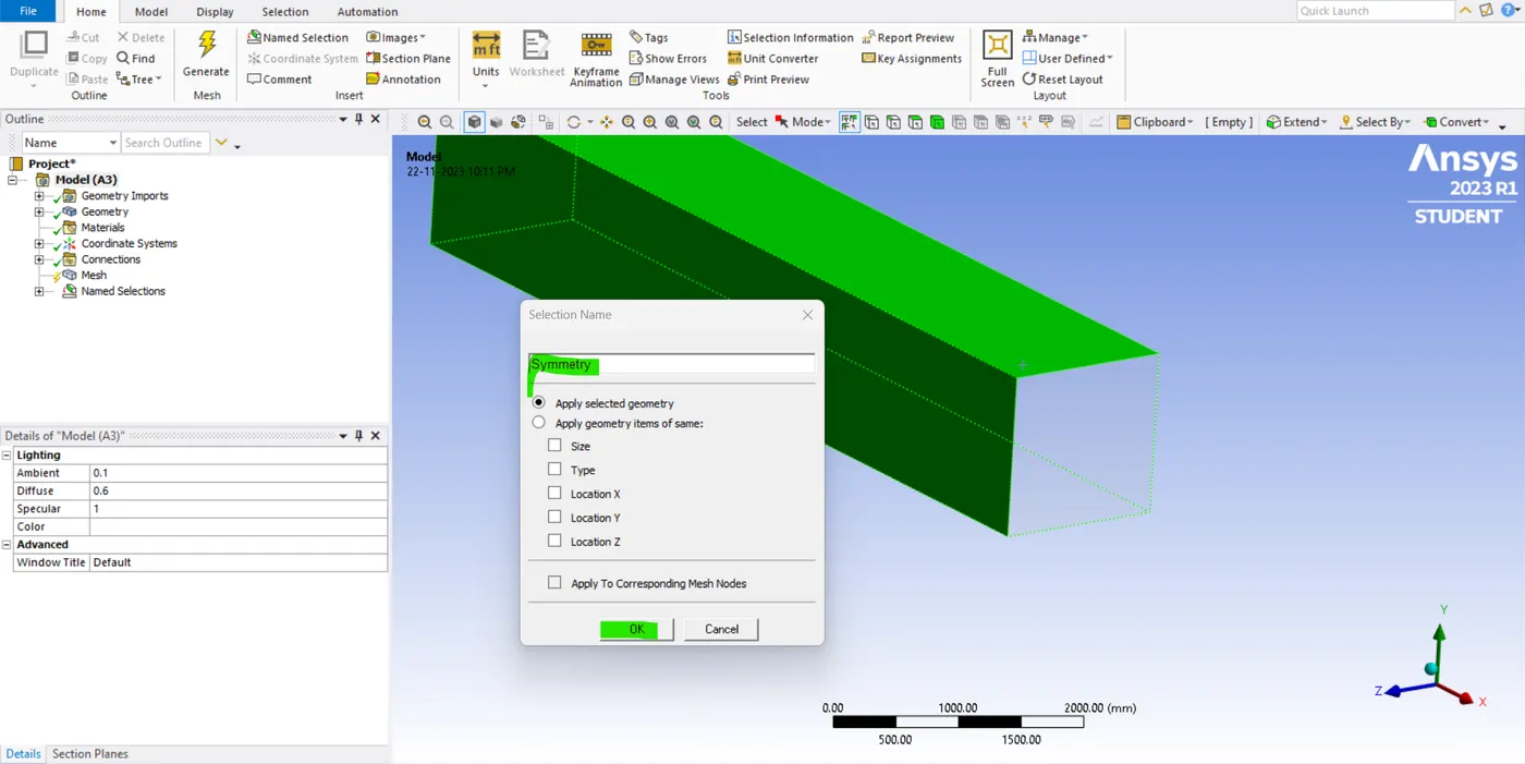
• so, After opening the meshing interface, I'm going to first use then press the "N" shortcut key. and I'm just going to call this the "inlet". Similarly except for inlet and outlet and Ahmed's body face. select the remaining face and name as the symmetry-wall.

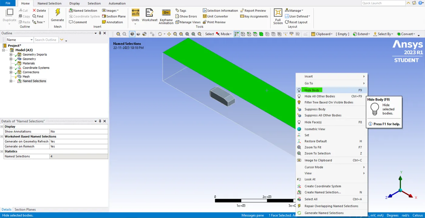
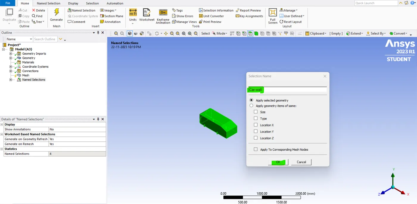
• Now we need to hide the entire face except Ahmed's body. so, to do that select the face and hit the "f8" shortcut key. now the faces are hidden. Similarly, we need to hide the entire face except Ahmed's body. so, after hiding all the faces we need to box select the Ahmed body and name it the "car model".

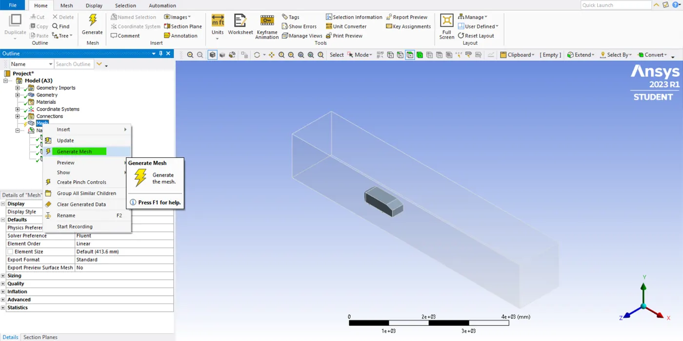
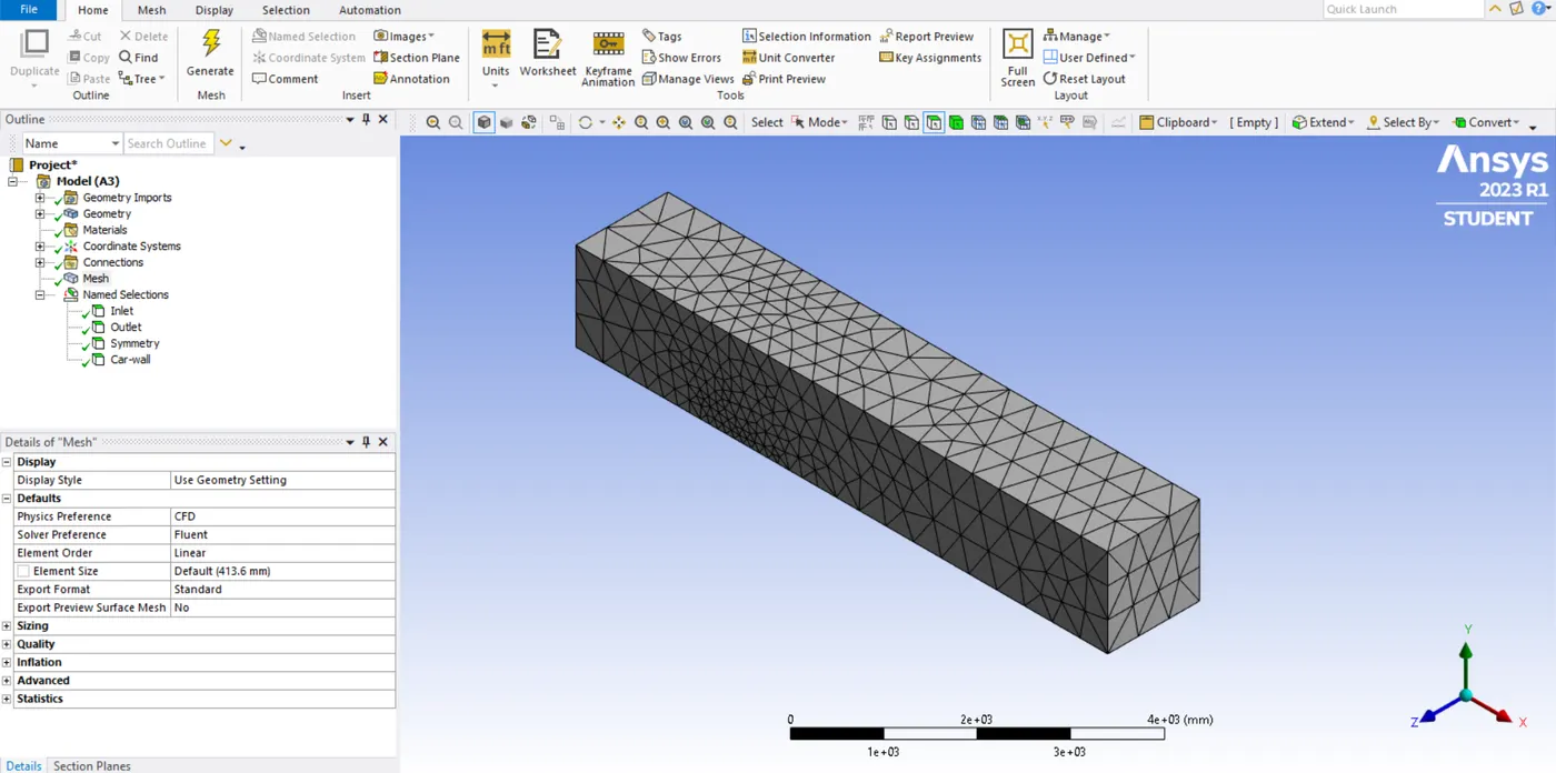
• So, after naming the faces and body. now what we need to do is we need to click on mesh and right-click to generate mesh. now the mesh has been generated.

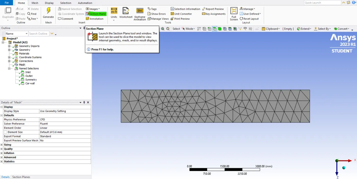
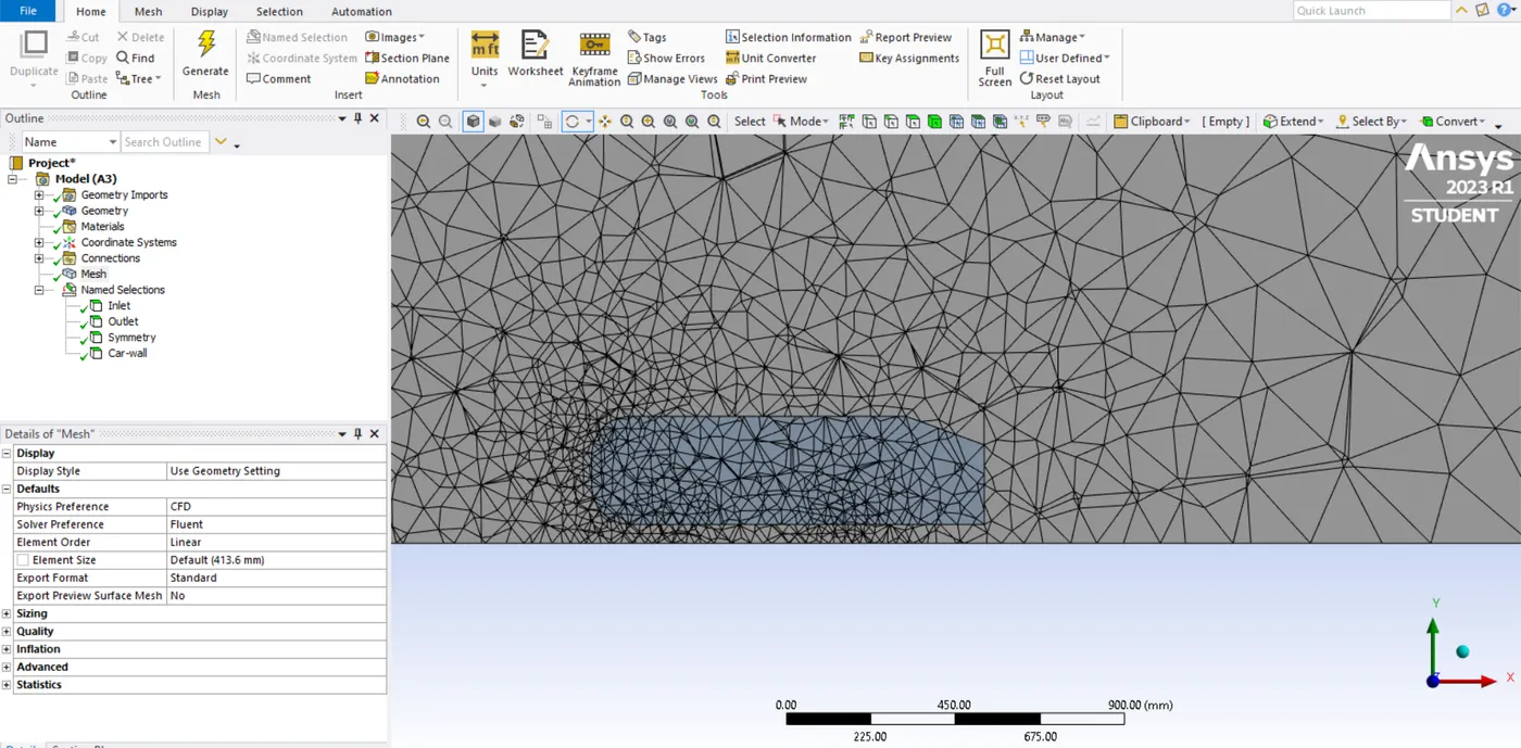
• now we need to look at the inside of the enclosure and Ahmed's body. so, to do that I'm going to cut this guy open. now when we see this you can see that mesh has been generated but we are seeing the mesh inside of Ahmed's body. now this does not look good. because we have the mesh in a region. where we don't want to simulate the flow.

• We don't want to see any type of computational mesh inside because the analysis is going to be done, only the flow outside of the Ahmed body matters. so, we have to fix this to this go back to the space claim.
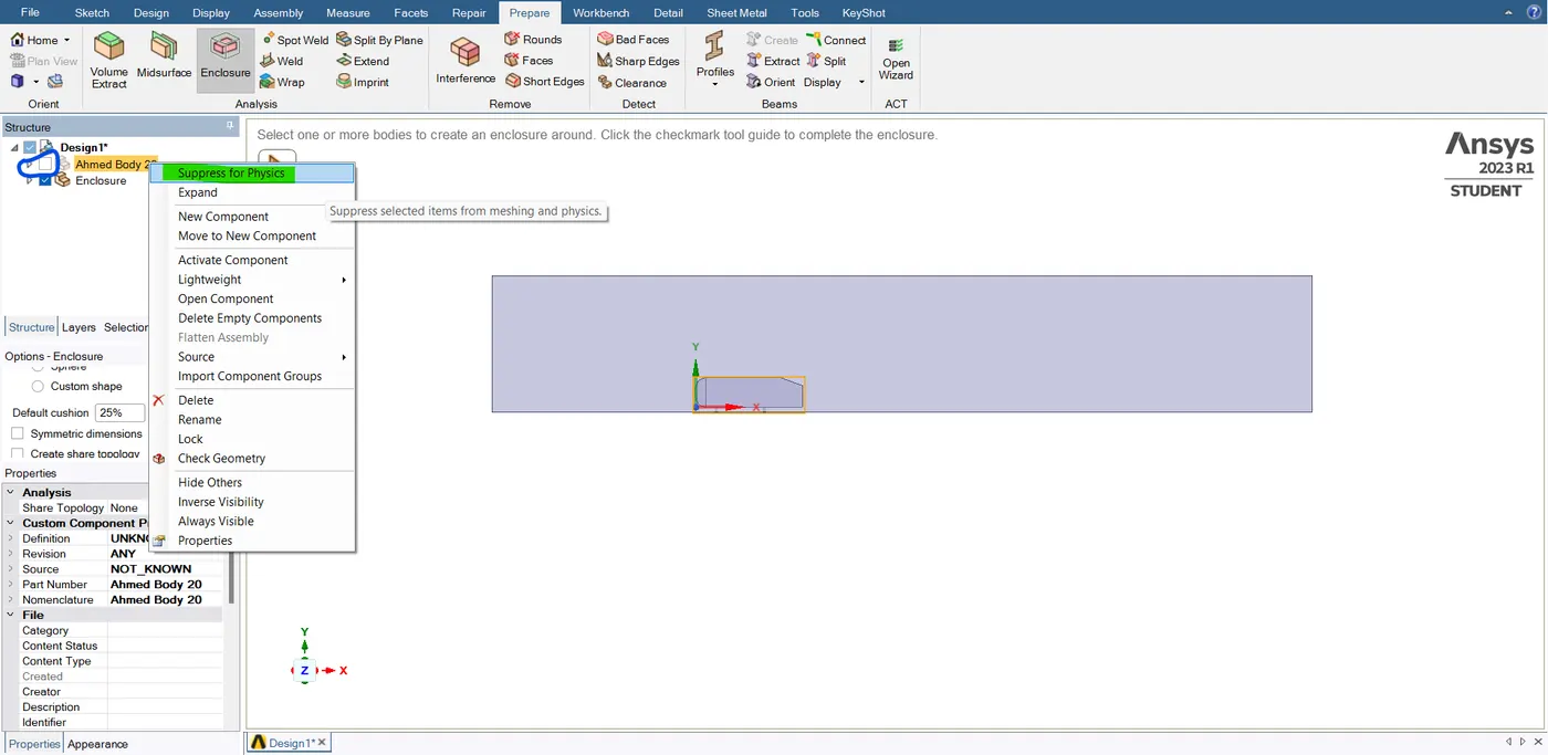
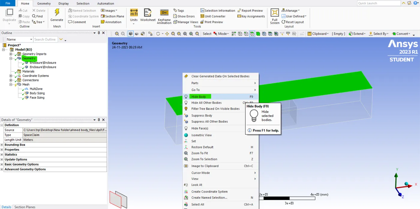
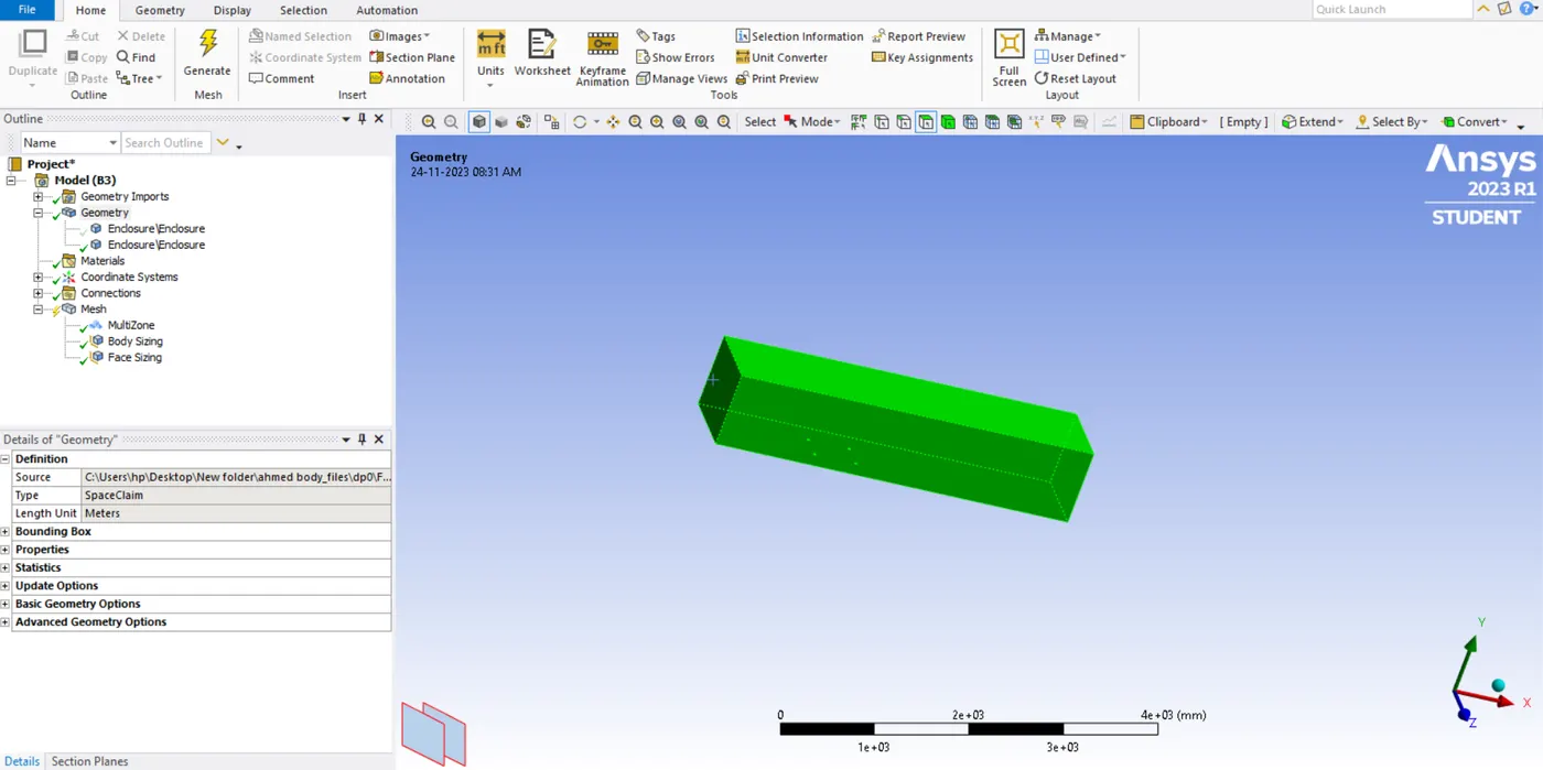
• And now the geomentry space claim is opened. so, the reason this is happening is we have two copies of this Ahmed body. so, this is causing the issue. so, now I'm going to hit right click and select suppress for physics in the Ahmed body and close this geomentry. and now go to mesh again.

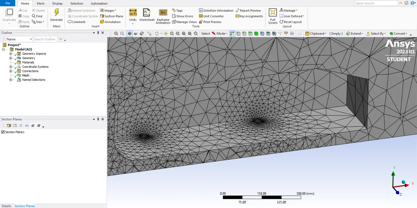
• after opening the mesh GUI. Now generate the mesh again but before doing this erase the previous mesh. now the mesh is generated and if I zoom in to see the geomentry. everything is captured correctly and this is exactly what we need to run this simulation.

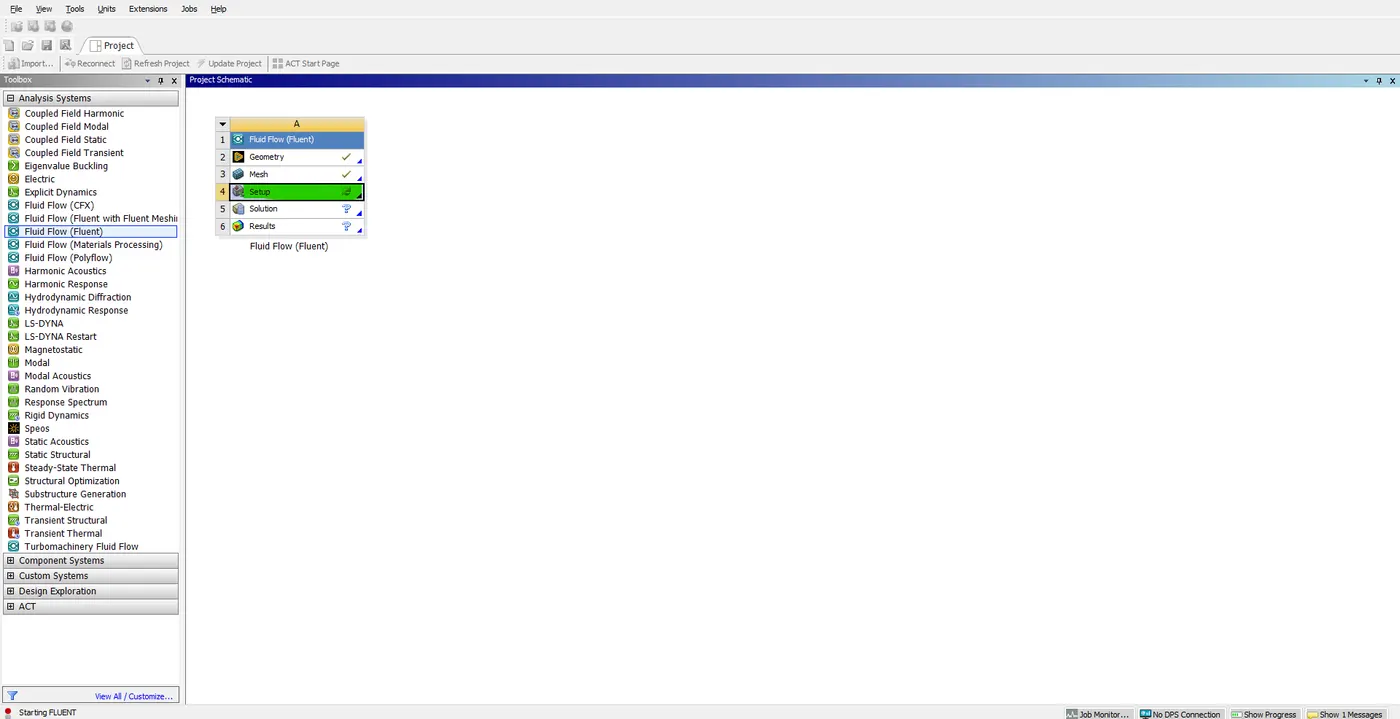
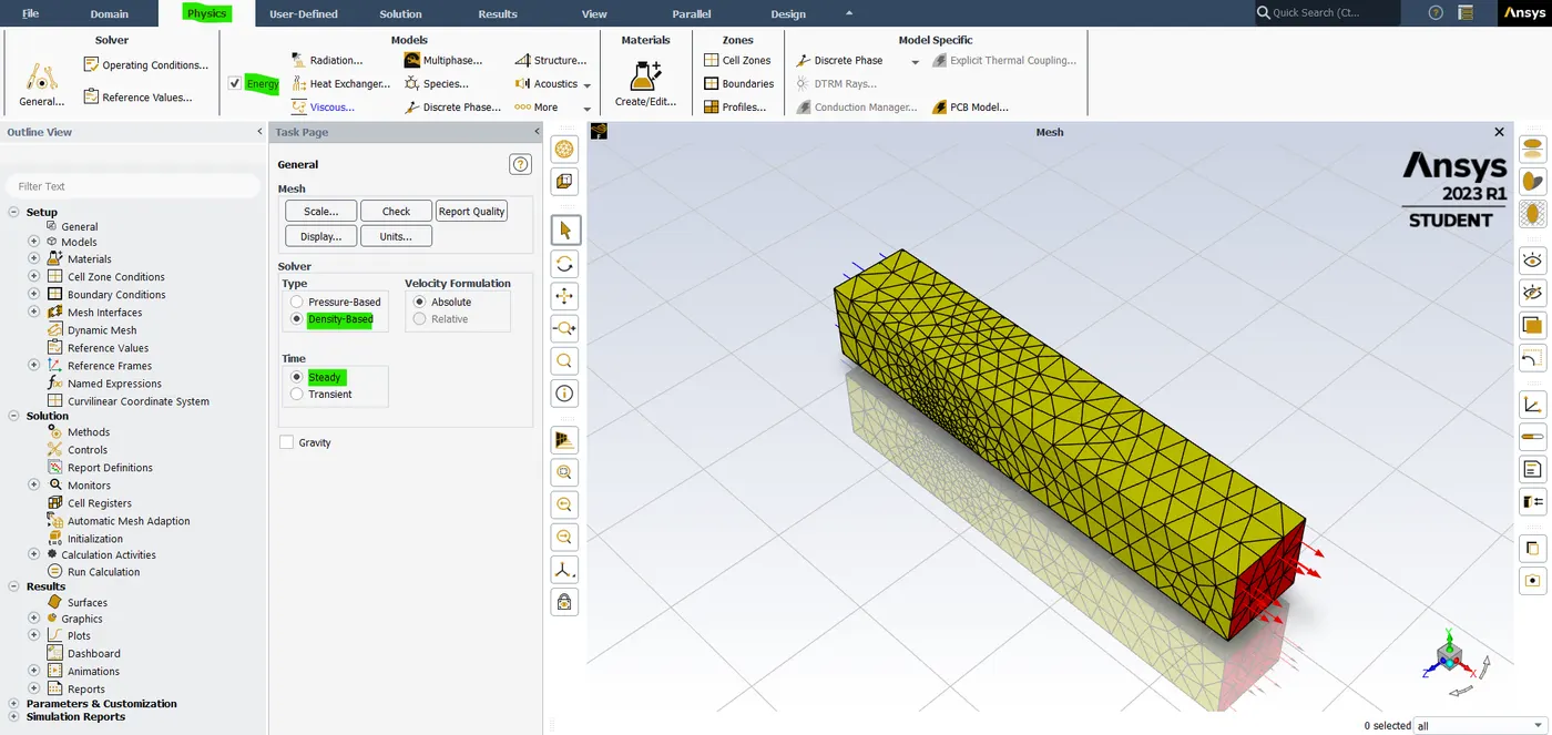
• now close the mesh GUI and update the mesh interface. after that open the setup interface, just go to setting up physics and select the solver type "density-base" solver and the timer is "steady". so, in this case, the inlet velocity is 25 m/s from the mag number point of you it's not a lot from the speed of sound it's just 340. but for convenience assume 300 m/s. In our case, the inlet is going to be 25 m/s. maximum we are looking up the value is 1/6. so basically the max number in this point of you is 0.3 or slightly lower than that. but whenever the max number is 0.3 or above it's good to use density base solver. because we need to take into the good compressibility effects so that's why in this case we are using a "density base solver".
• And in the time state we can use both the steady state and transient state of the solver. but in this case, we are interested in looking at what's the "Drag force" on the car and what's the "velocity distribution" in the rear end of the car what the wake looks like, and the kind of stuff. so, we are ok with the steady state. so, let's go with that.

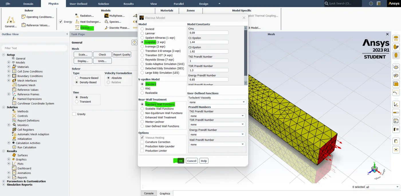
• So, we set the physics and in this case, the viscous model is we are using the "turbulence model". so, I'm going to use the k-epsilon and that's going to be the initial choice of turbulence model and this is not a good one for this model. but we just using after that click "OK".
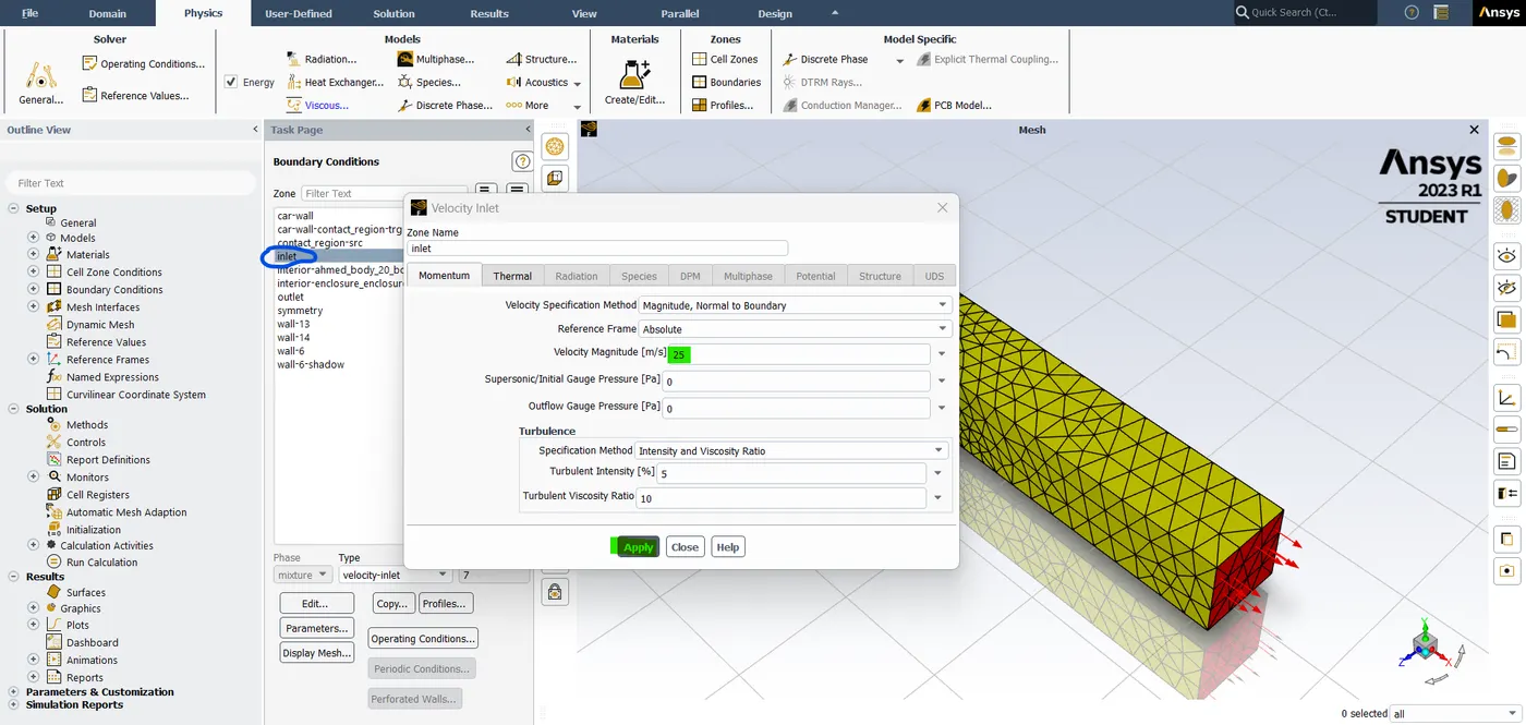
• In this case we are using an energy equation turned on. and the material is air. then let's go to the boundary. and select my inlet type is automatically flagged as a velocity magnitude is 25 m/s and the thermal is 300(k). click "OK".

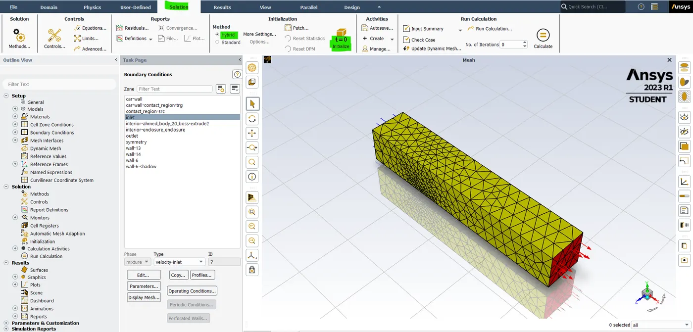
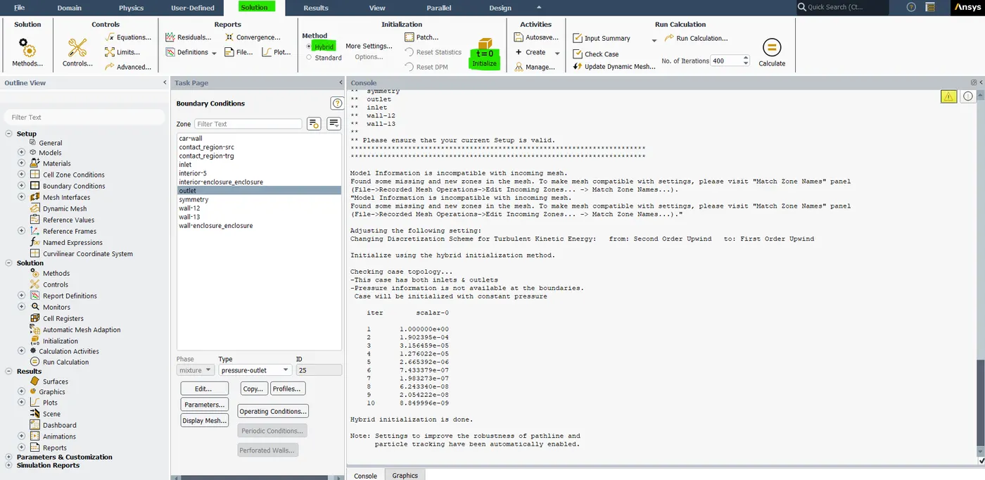
• And if I look at the symmetry wall the type symmetry is applied and the outlet gauge pressure is 0. so, we are ready to solve the problem. so, the first initialization of the method is hybrid. when we apply the hybrid initialization it uses the potential flow solver which means we compute the two variables called "distributed function" and "velocity potential" which automatically satisfy the continuity equation.
• but the idea is we can solve the potential variable and get an estimate of the initial velocity. so, it provides an excellent initial condition or starting point. it's not accurate but it gives a very good starting point. and sometimes the flow path is very complex. for example, a centrifugal pump might be handy. we get PDE that will solve iteratively and that is what happens when I hit initialize.
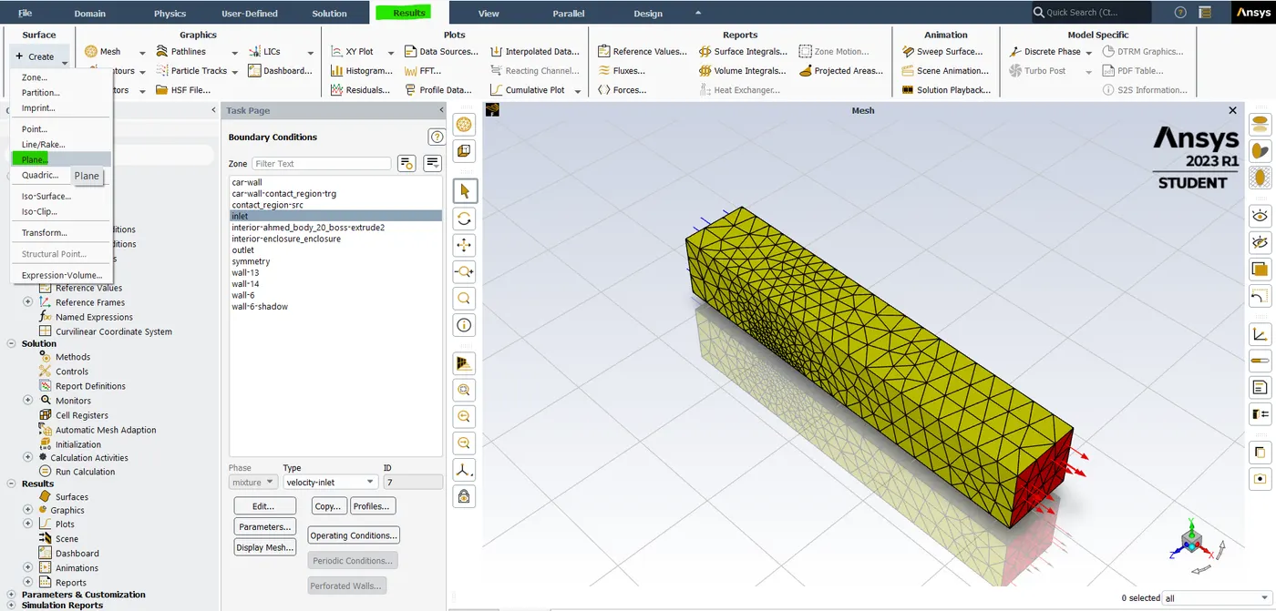
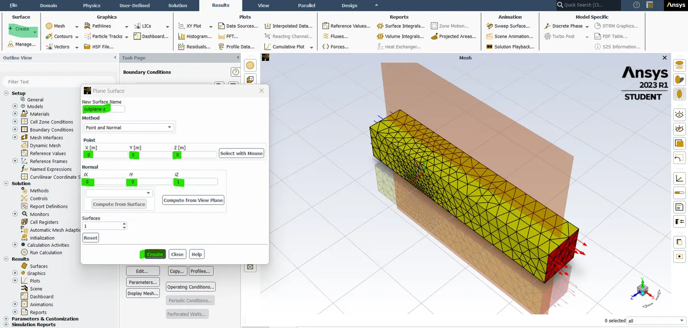
• Now I'm going to the postprocessing section and we are going to create a cut plain in the z-axis to see how the velocity looks this is something that we want to monitor as the simulation is running. so, let's go to the "create" option -> select the "plain" option -> In that select point and normal option. so, the points in x=0, y=0, z=0, and in normal the ix, iy=0, and the iz =1. name it as a cut plan z and hit the create option.

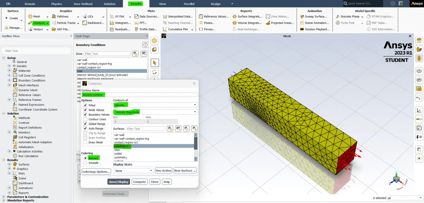
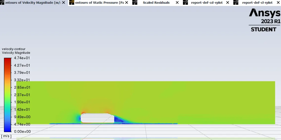
• and then now just go to "contours" and click on "new". so, In that select the contours of "velocity" and "velocity magnitude". and select the "cut plan z". it was named a velocity contour hit save and display.
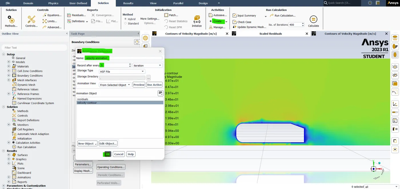
• Now we need to create a solution animation. so go to "solution animation". name as a "velocity animation" set the view of the model hit "use active" and select the animation object as "velocity contour" Click OK.

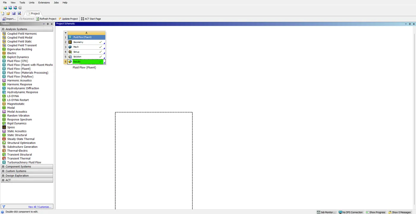
• so to start with 500 iterations in run calculation and hit calculate. so, once it is completed after opening the CFD Post-processing and closing this setup GUI.

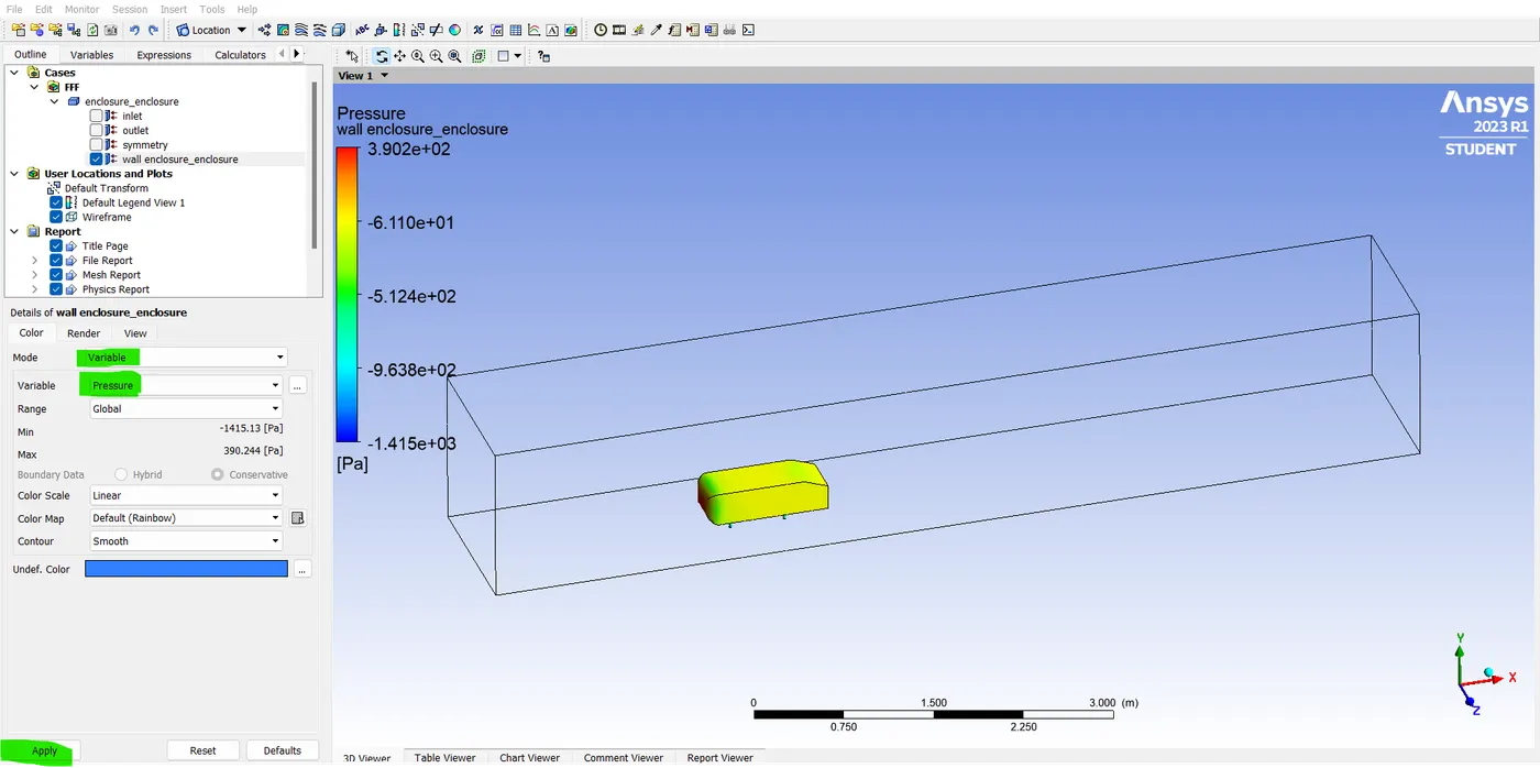
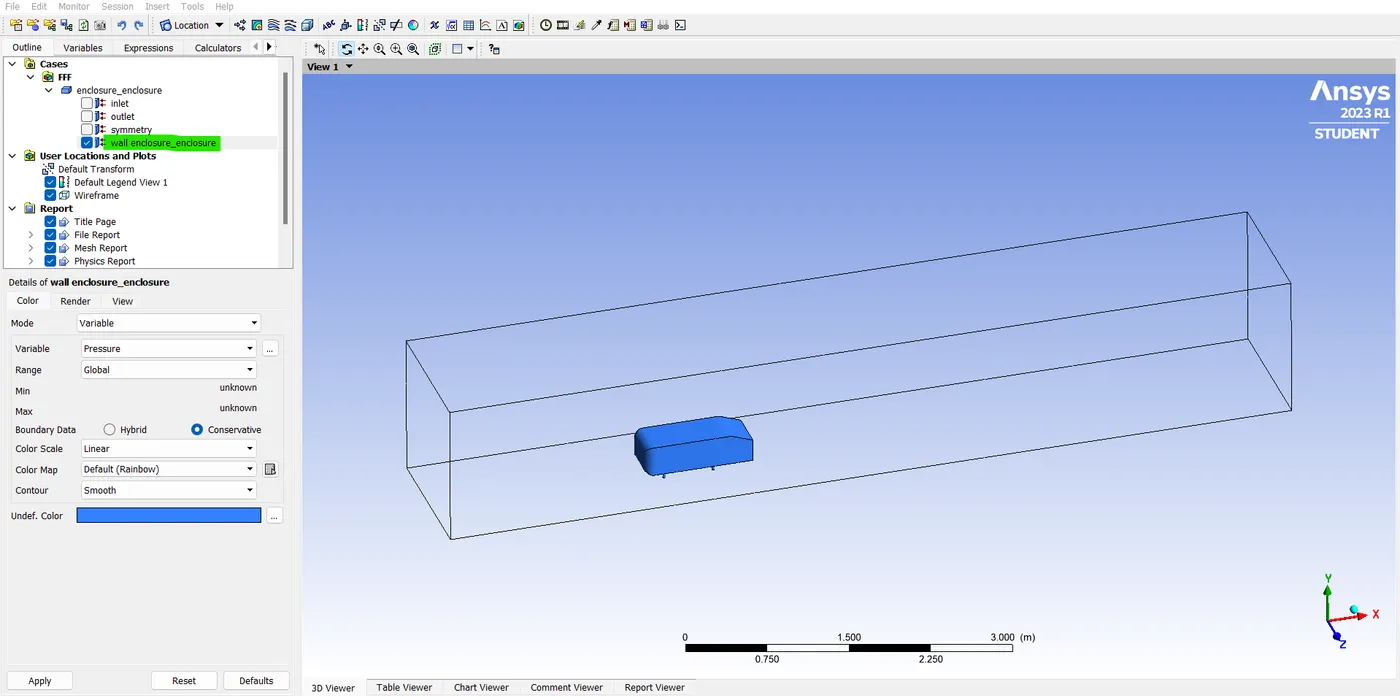
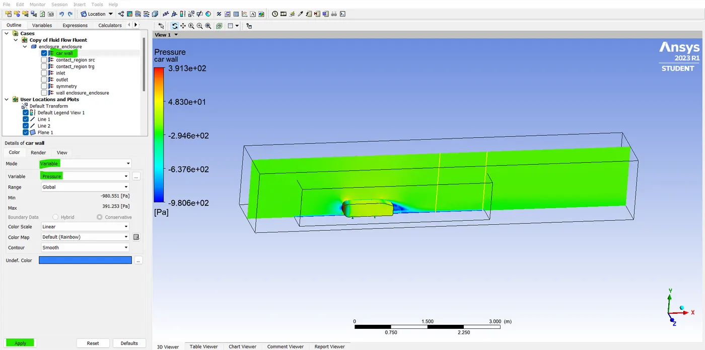
• After opening the result section. now you can see the geomentry is loaded. so, double-click the "car-wall" and change that mode into "variable" and change the "variable" into "pressure" and hit apply.
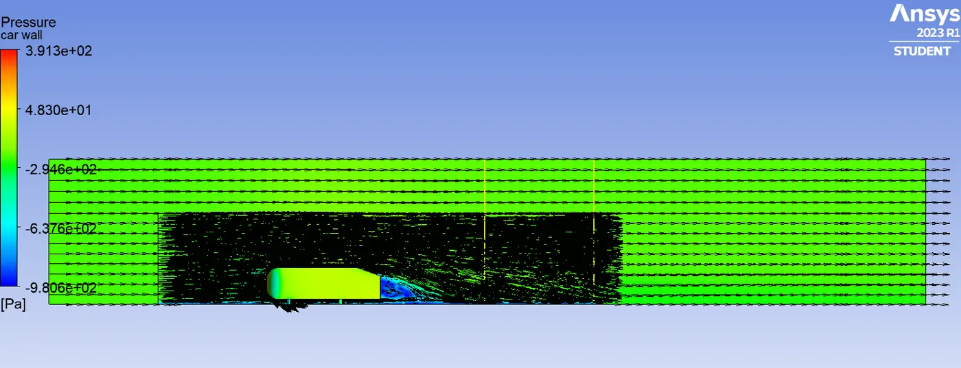
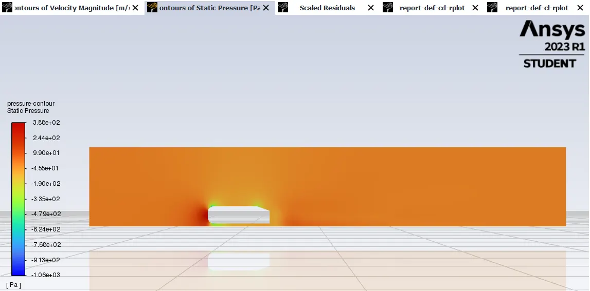
• so now we can see the pressure applied in the body. in the front side of the car, the pressure is 1.561e to 3 and then these are areas that were going in negative.
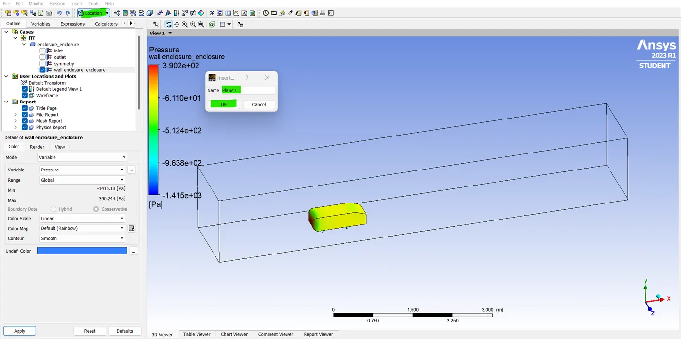
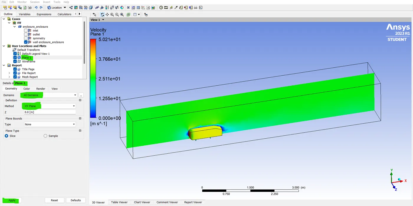
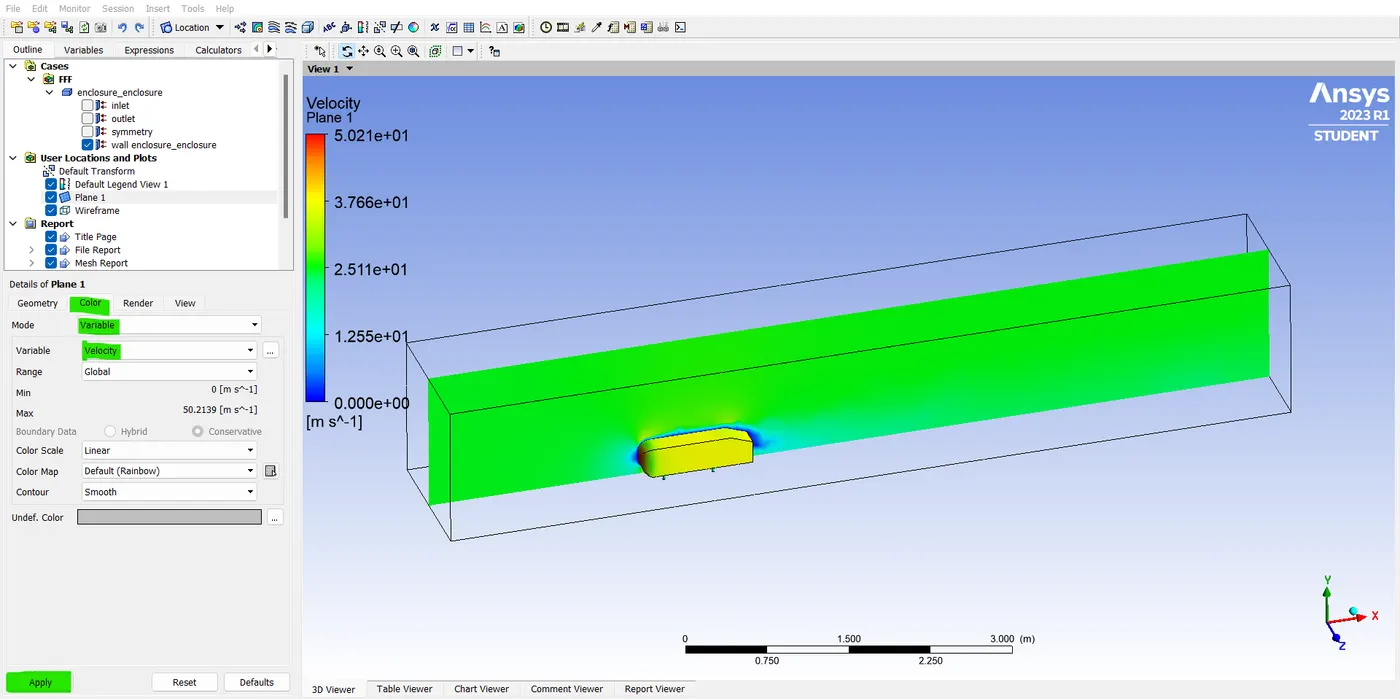
• so, now goto "insert"->"location"-> "plane" -> and name the plane as "cut plane z". and in the method we need to select xy plane and click "apply". and in color apply "velocity" in variable and hit "apply". and in render enable the "show mesh line" option hit "apply".

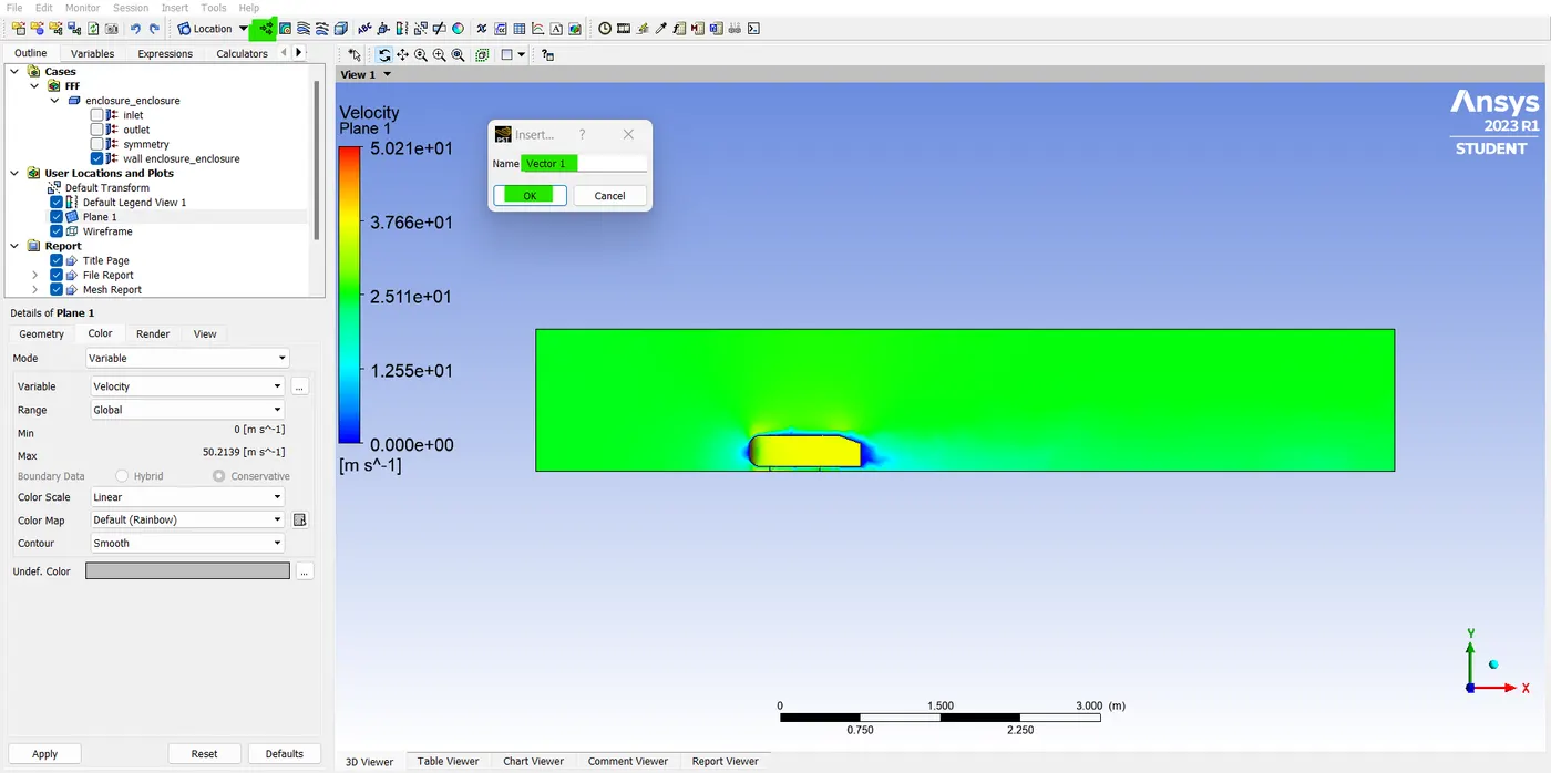
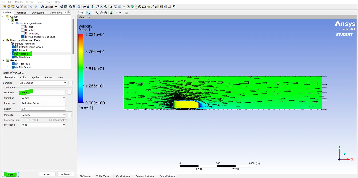
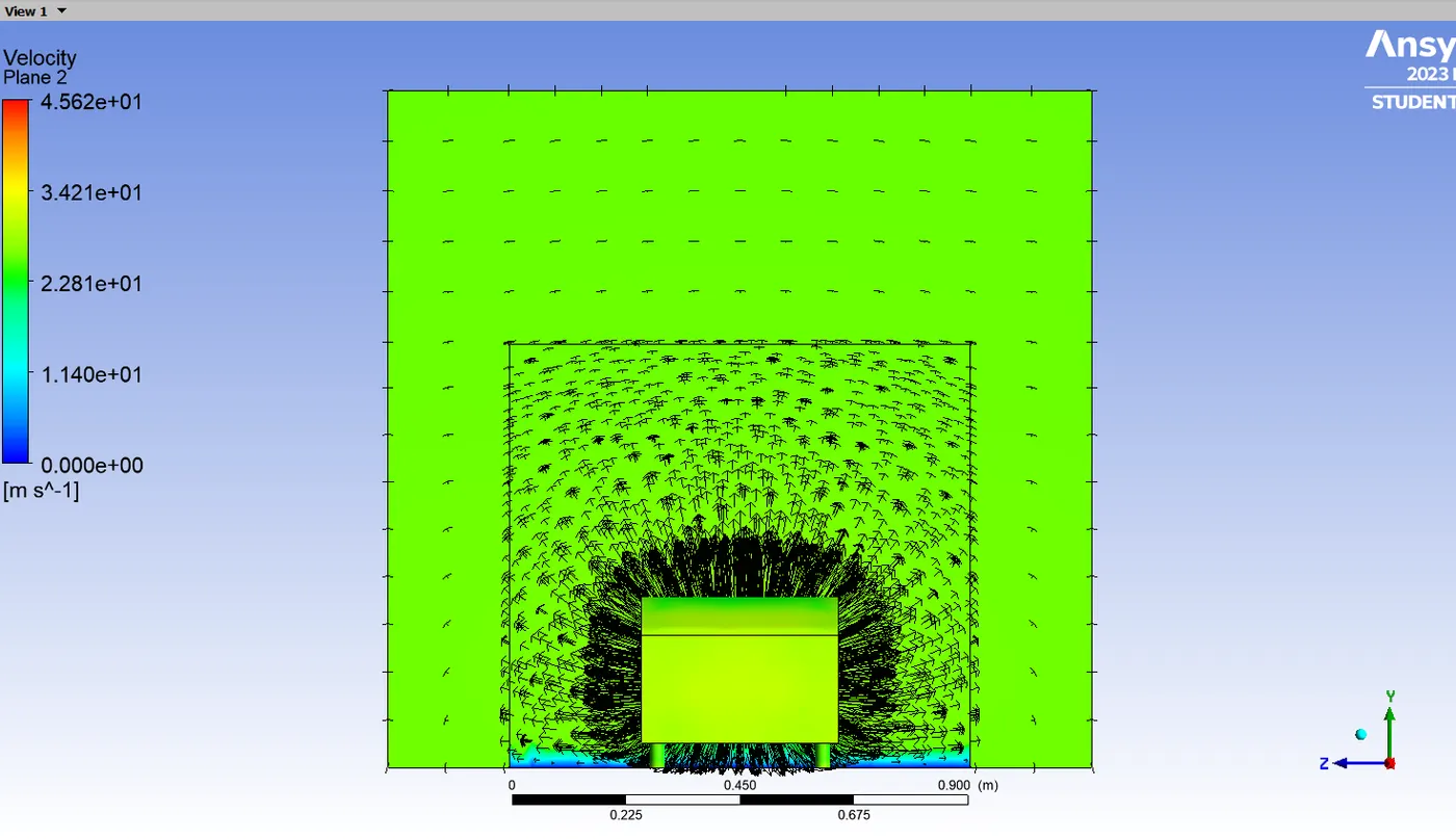
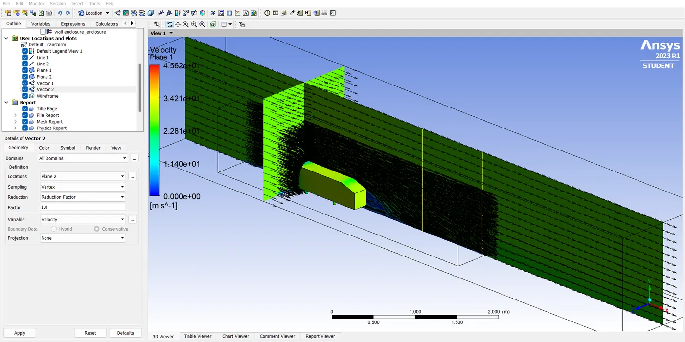
• so, now we can see the Ahmed body result the backside of the Ahmed body has a wake region the velocity is getting lower here and now, we need to create the "vector plots" and color them in "black". in geomentry select the "cut plan z" in "location" and hit "Apply".
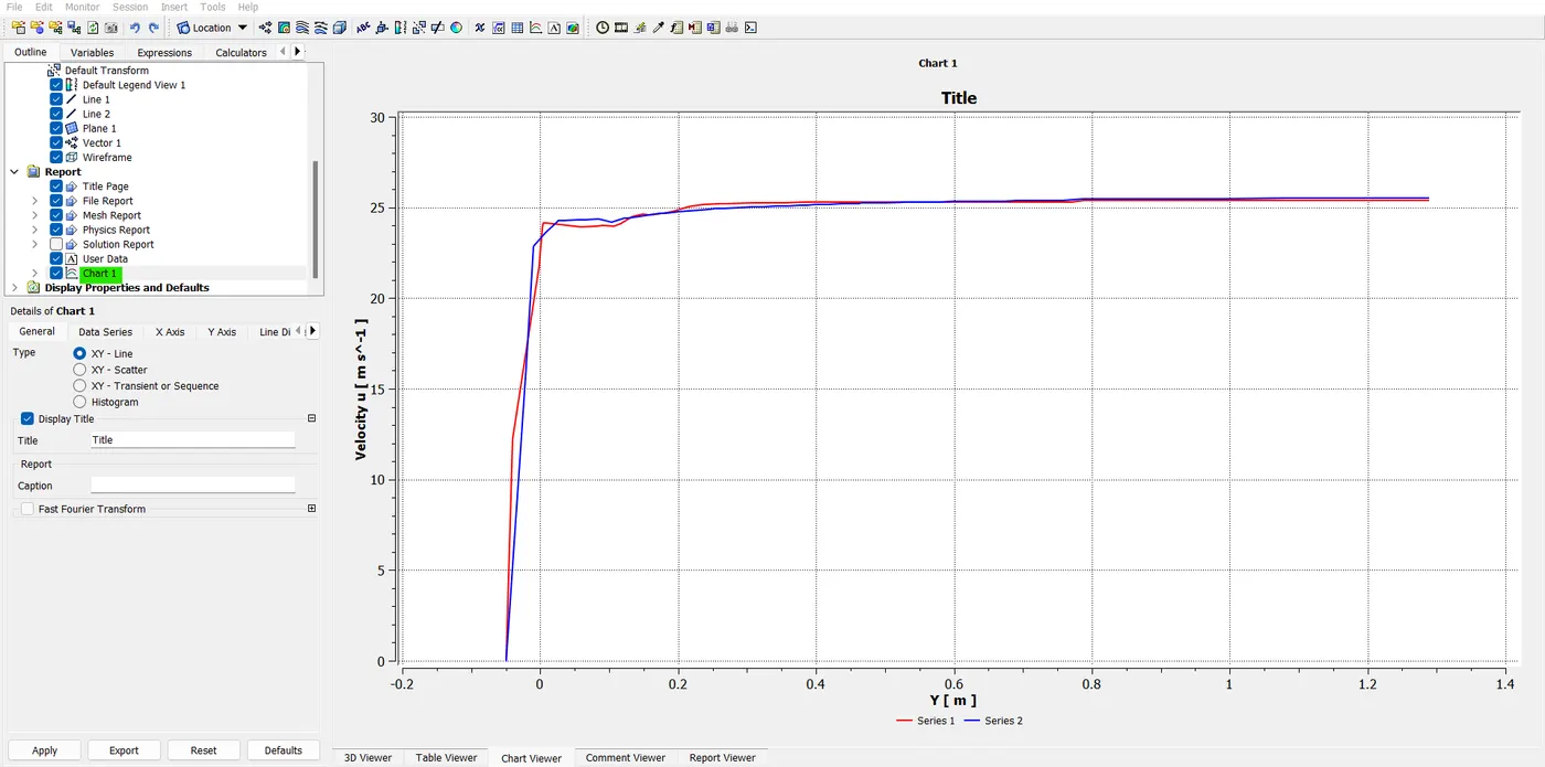
• In actual Experimentation of what they did the velocity is in several vertical stations. so, you can think of having a link after the Ahmed body and before the Ahmed body and also on top of the Ahmed body and along that line is measuring velocity. so, you will get a very nice velocity profile.

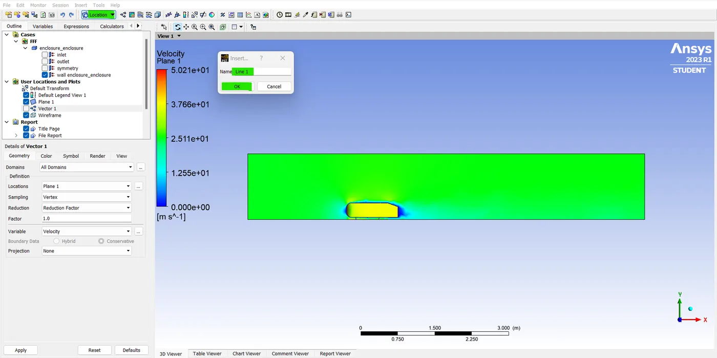
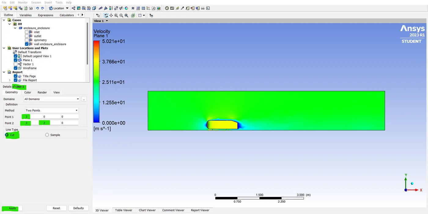
• so, to do that deselection the vector plot and go to "Insert" -> "Location" -> "line-1". This line is going to be created now in definition point 1 is 200 point 2 is 220. and the line type is "cut". the cut is cut the domain and get the data.

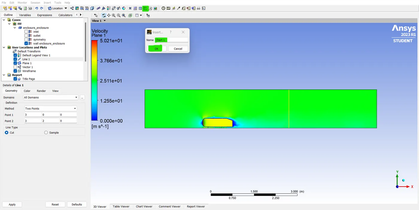
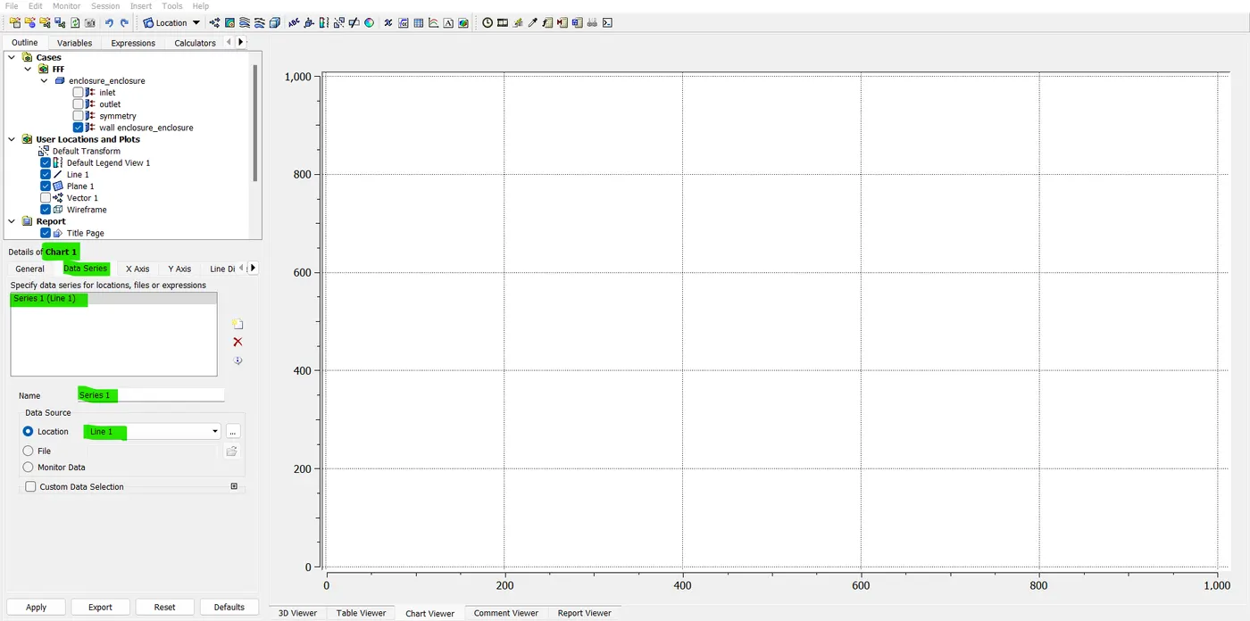
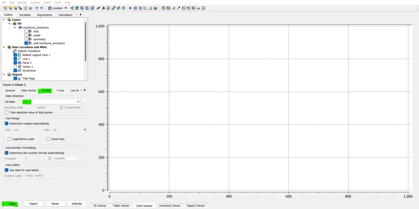
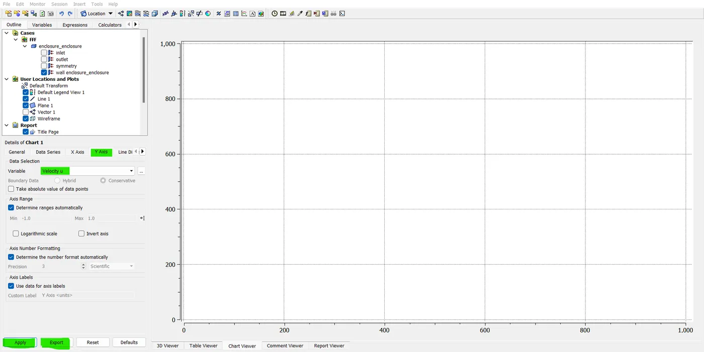
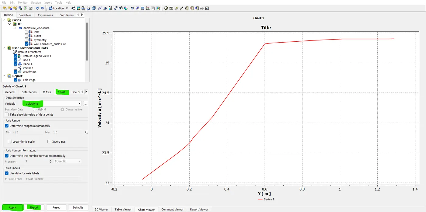
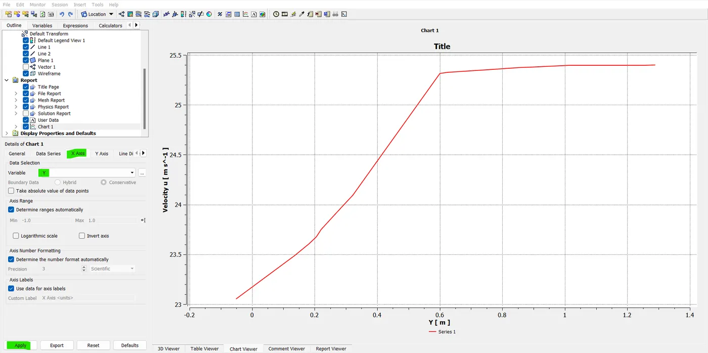
• now we need to insert the chart go to the "insert" option -> "Location" -> "chart-1". so, this is going to be the xy line chart and the data series. select "line 1" in location "data series". For the x-axis, the variable would be in y, and for the y-axis, the variable would be in velocity u and then hit "apply".

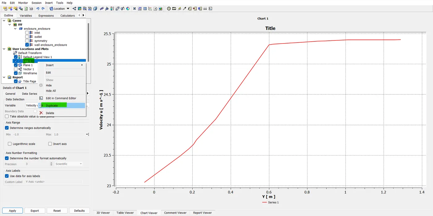
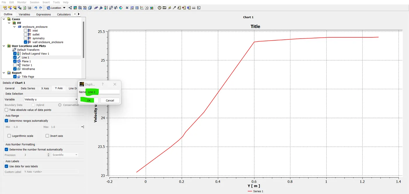
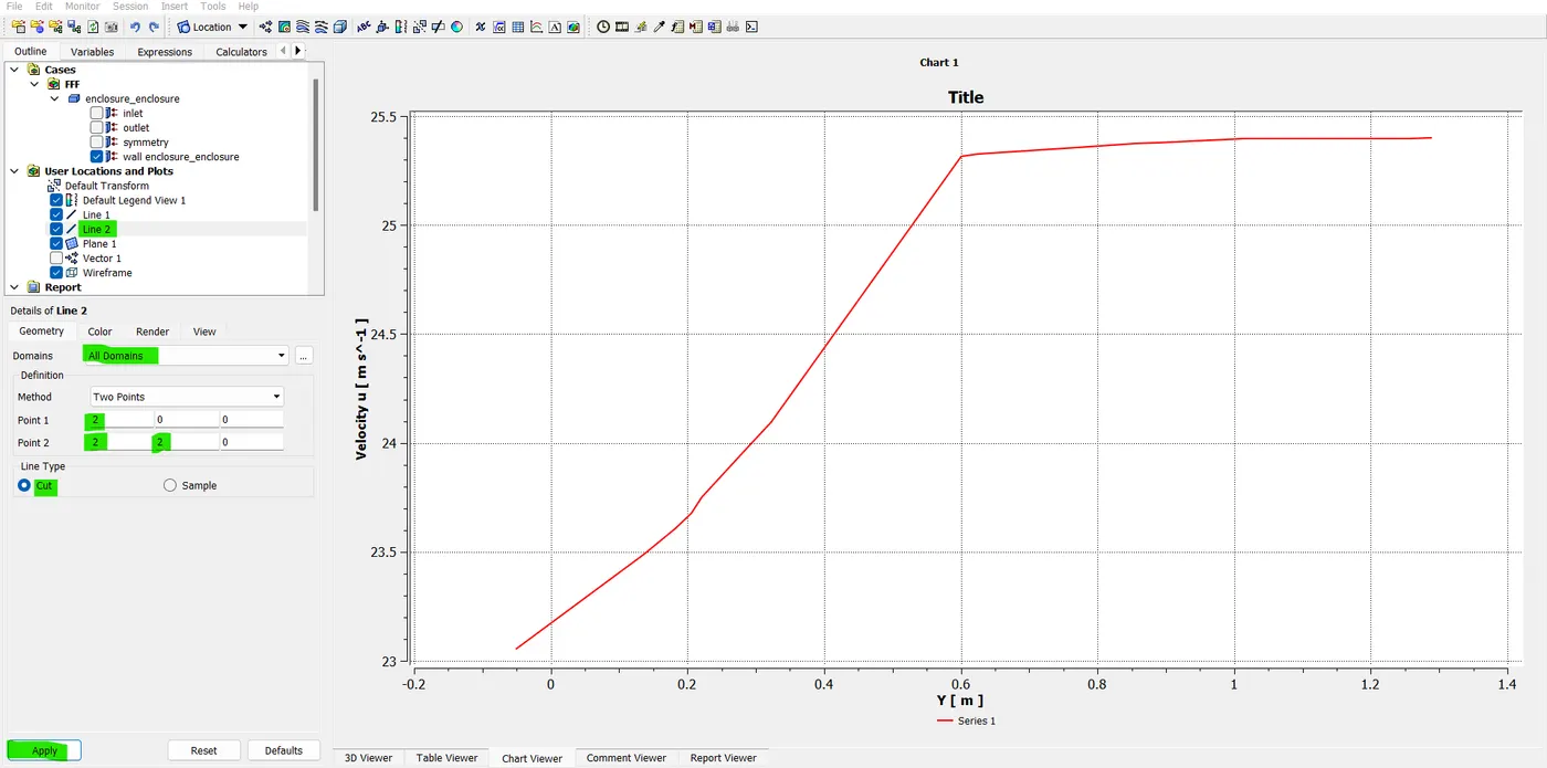
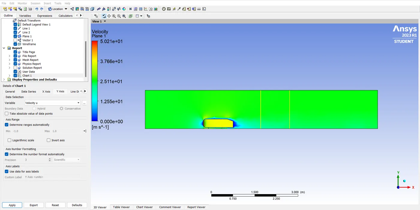
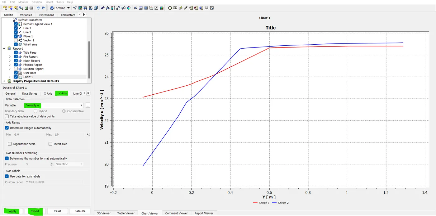
• now you can see the velocity profile is in that line. Now we need to duplicate line-1 and name it as line-2. and in line 2 change the coordinate into 3 in both points 1 and 2. Hit apply and you can see in the 3D viewer there are 2 sets of lines.
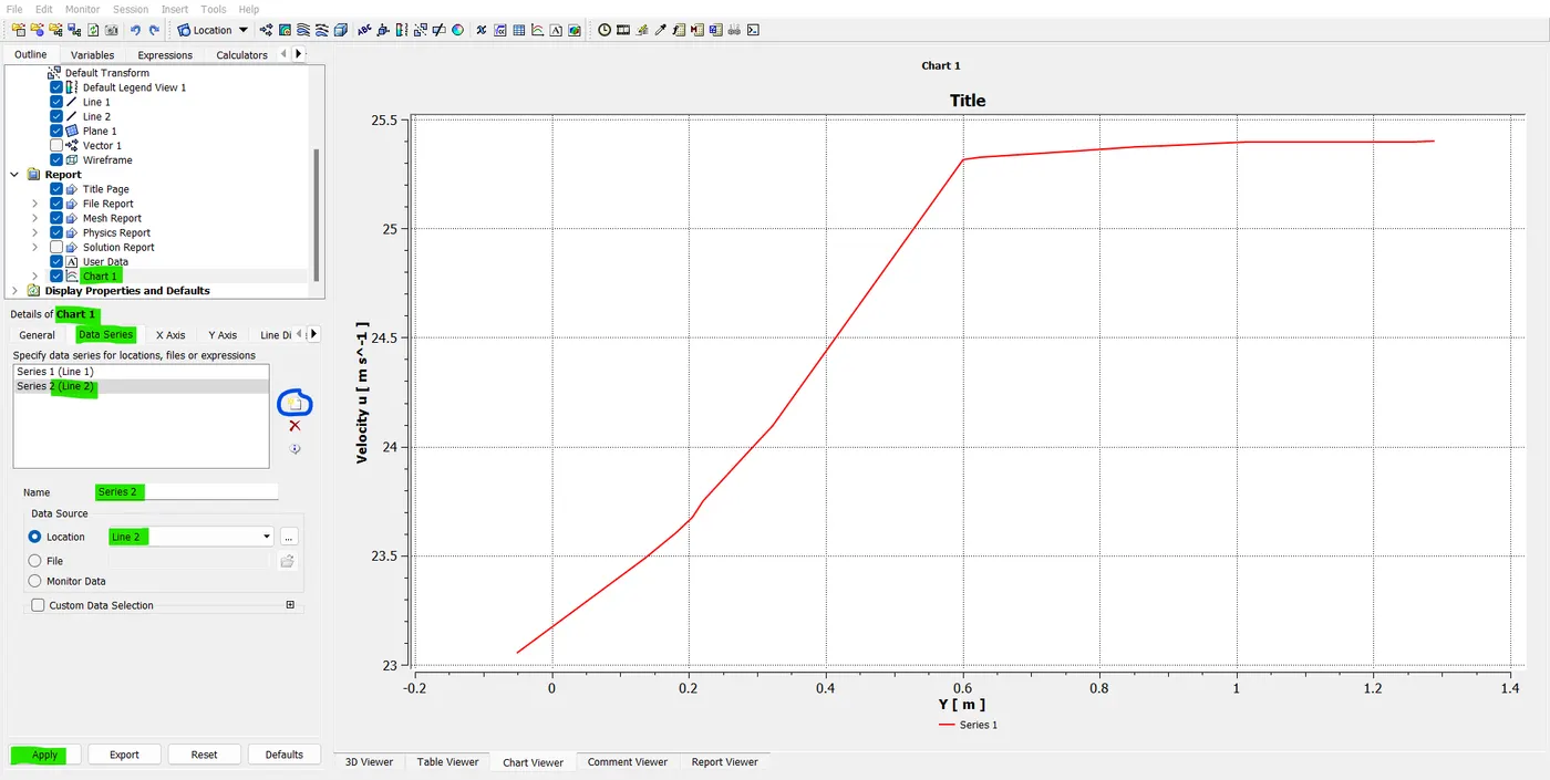
• Again go to chart-1 go to data series and click "new" data series this is going to be line-2 in location and hit apply. now you can see in my chart there are two curves in a single chart.
• And then export the chart. so, save the chart into the document and then open it in Excel save the file name as "data from CFD post" and hit "save". Then open the document in Excel. So, here we have the y value of the velocity and the u component of the velocity for that particularly in the Excel sheet, and we have both the lines problem.
• so, this is greater because now we can run a bunch of experiments to make our mesh finer. also, we can compare how the velocity profile is affected for every chance that we make.

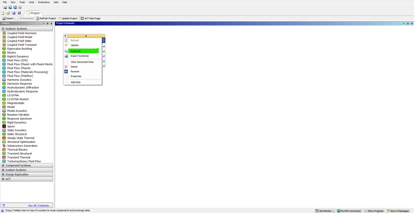
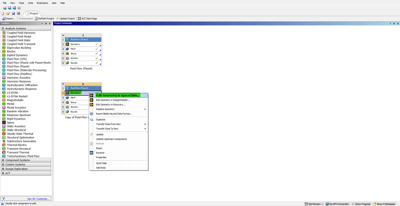
• so, now we just duplicate our setup here and name it an "Ahmed body refind setup". so, after that open the geomentry GUI. so, here you can see that in front of the Ahmed body and the wake region we saw the flow near the Ahmed body was high unresolved which means there are not lots of mesh points.
• so, now there are not lots of mesh points. so, now we are going to draw a box and refine the mesh much more finer inside the box instead of meshing the complete domain so, this is called local refinement.
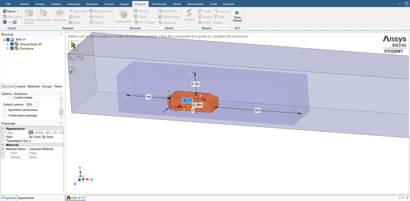
• so, to do this we need to select the "base-Extrude" and go to the "prepare" section and section "enclosure" option. so, you can see the box appear in this model. now the dimension is based on the wake region size seen in the baseline setup. so, when we run the simulation the wake might come outside of the box. which is bad. so, the way of calculating the dimension is upon the baseline setup and I need to make sure that the wake region is also refined.
• so, before giving the dimensions we need to uncheck the "symmetric dimensions" so, the wake region of Ahmed's body is 1 meter the circumference of the body is 0.5 meters. The bottom is 0 meters and the top side is 0.5 meters, hit "ok" and close the "geomentry" GUI.
• Now, before giving to the meshing Interface, we need to reset the mesh. why means, that there are no faces on the box only inside the box we can able to select. but we can see the name of the selection is the inlet and outlets. but we couldn't select that. so, we need to duplicate the case setup only if I do not change the geomentry a lot, which means say that the diameter or length of the particular feature then we can duplicate and save a lot of time. so, that's why the meshing interface is not playing well. so, now we need to reset the mesh.

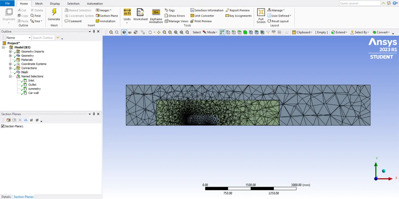
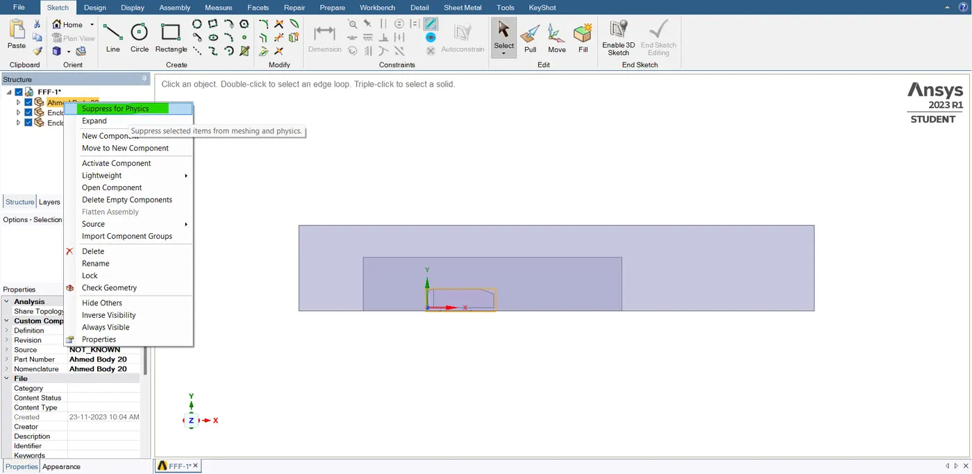
• so, after opening the mesh GUI. Now you can see that both the rectangle boxes are available. so, now first run the base-line mesh cut the section plane, and see what the mesh looks like. so, the internal geomentry of the mesh looks like this. s, the internal geomentry of the mesh is overlapped you can see the mesh from the internal box, and the mesh from the external box is not attached perfectly. so, this is bad, so to fix this we need to close the meshing interface. and go back to the geomentry interface.

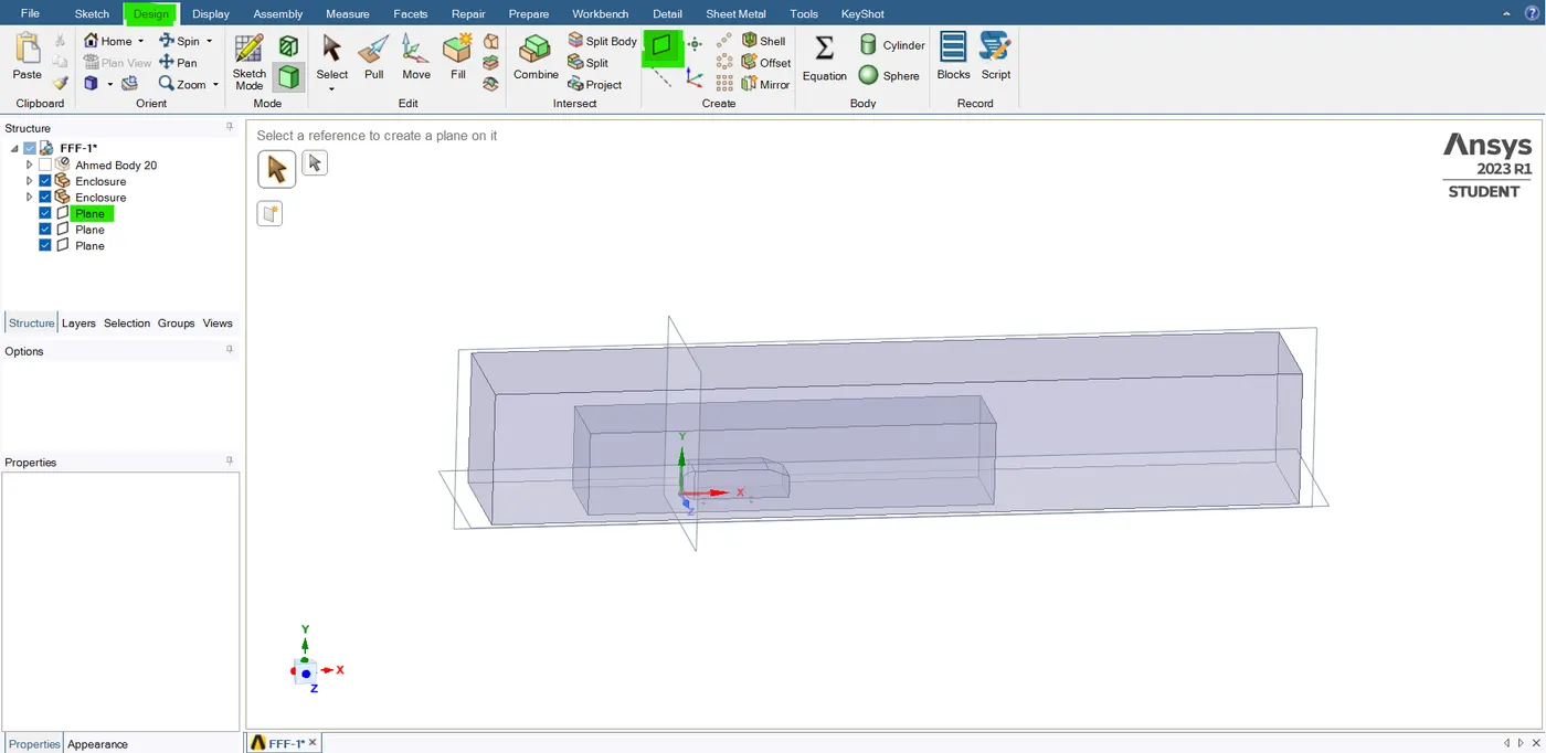
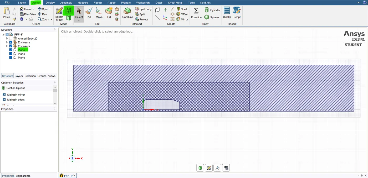
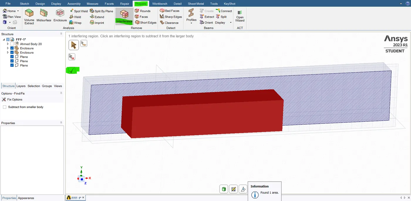
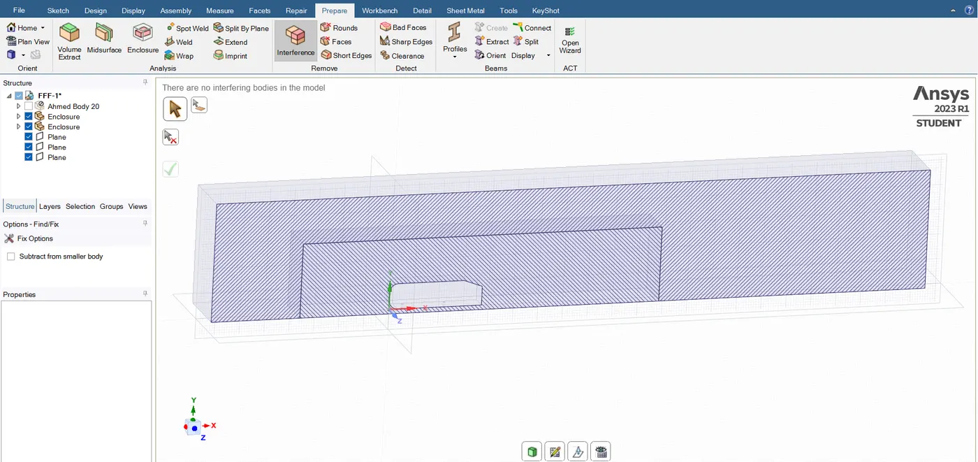
• first create the cross-section of the three planes in this model select the x-axis plane and then hit cross-section mode. so, now you can see the hatch patterns but in the smaller box, there are hatch pattern objects in both directions. so there are overlapped regions and we don't want that. so, to eliminate this problem go to the "prepare" section -> select the "interface" option -> and hit "ok" Now you see the problem solved. this does not overlap. so, close to the geomentry GUI.

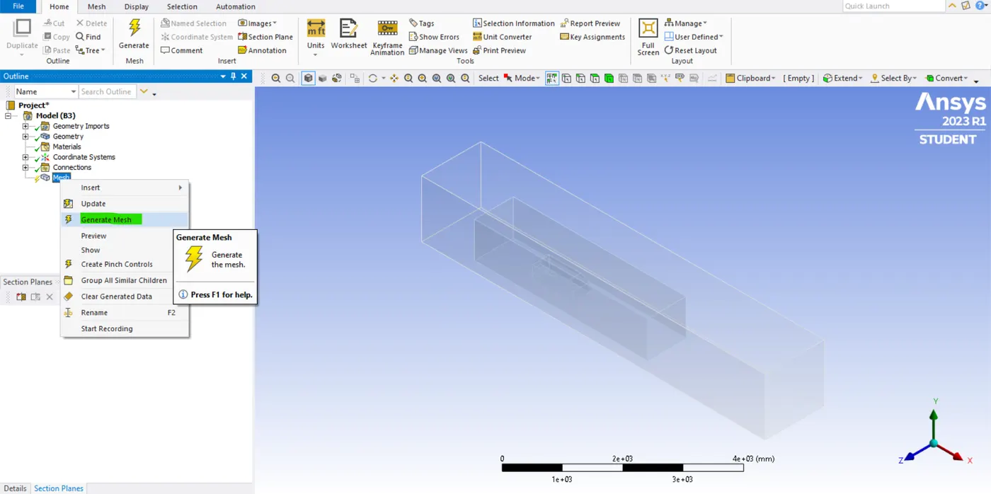
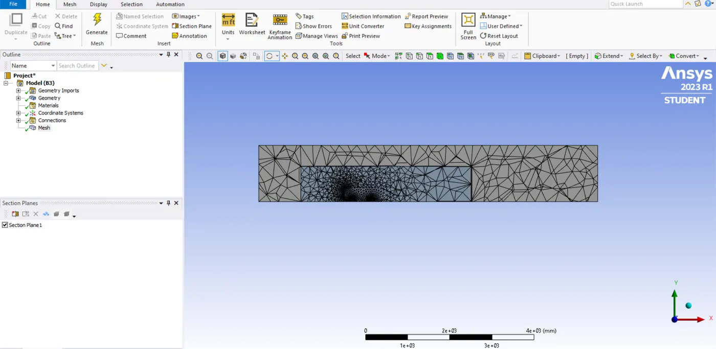
• New open the meshing interface and generate the mesh again and you can see there is perfect connectivity and no mesh overlapped. so, now let's work on the meshing part so, you can see the outside of the inner region there is a perface structure which means there are perface straight lines. so, even in this scenario it is better to use hexahedral mesh has quality of the all mesh types.

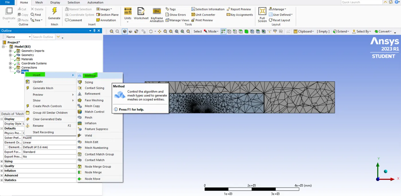
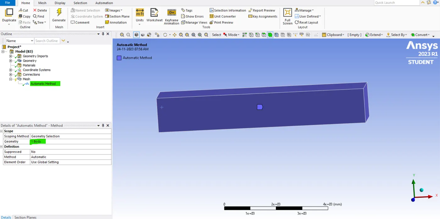
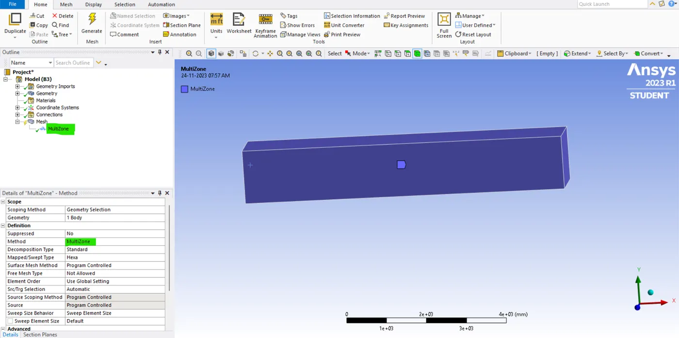
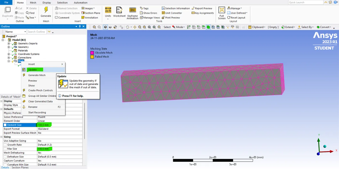
• so, to do this click on "mesh" and select the automatic method. so, the method is used to select the entire body and hit "apply". and in the "method" -> use "multizone". the multizone is going to try and create a hexahedral mesh wherever possible and in the other region, it's going to connect perfectly.
• Enter the " element size 100mm" and in the "sizing section there is a max size that is also 100mm". so, it represents the evenly sized mesh in the outer region. finally, right right-click mesh and update the mesh.

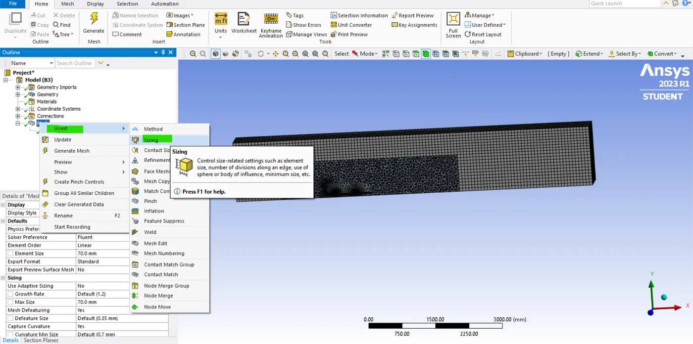
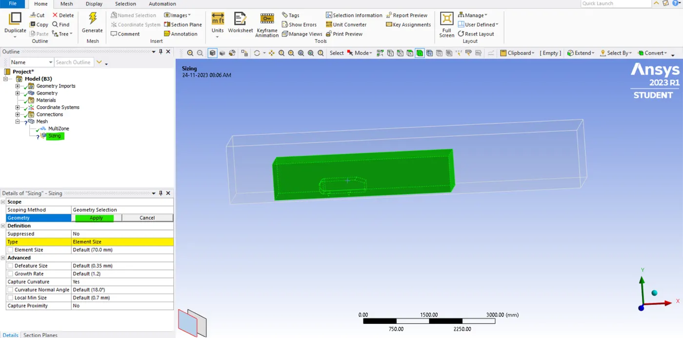
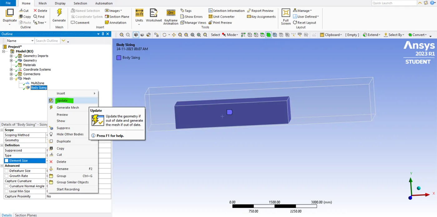
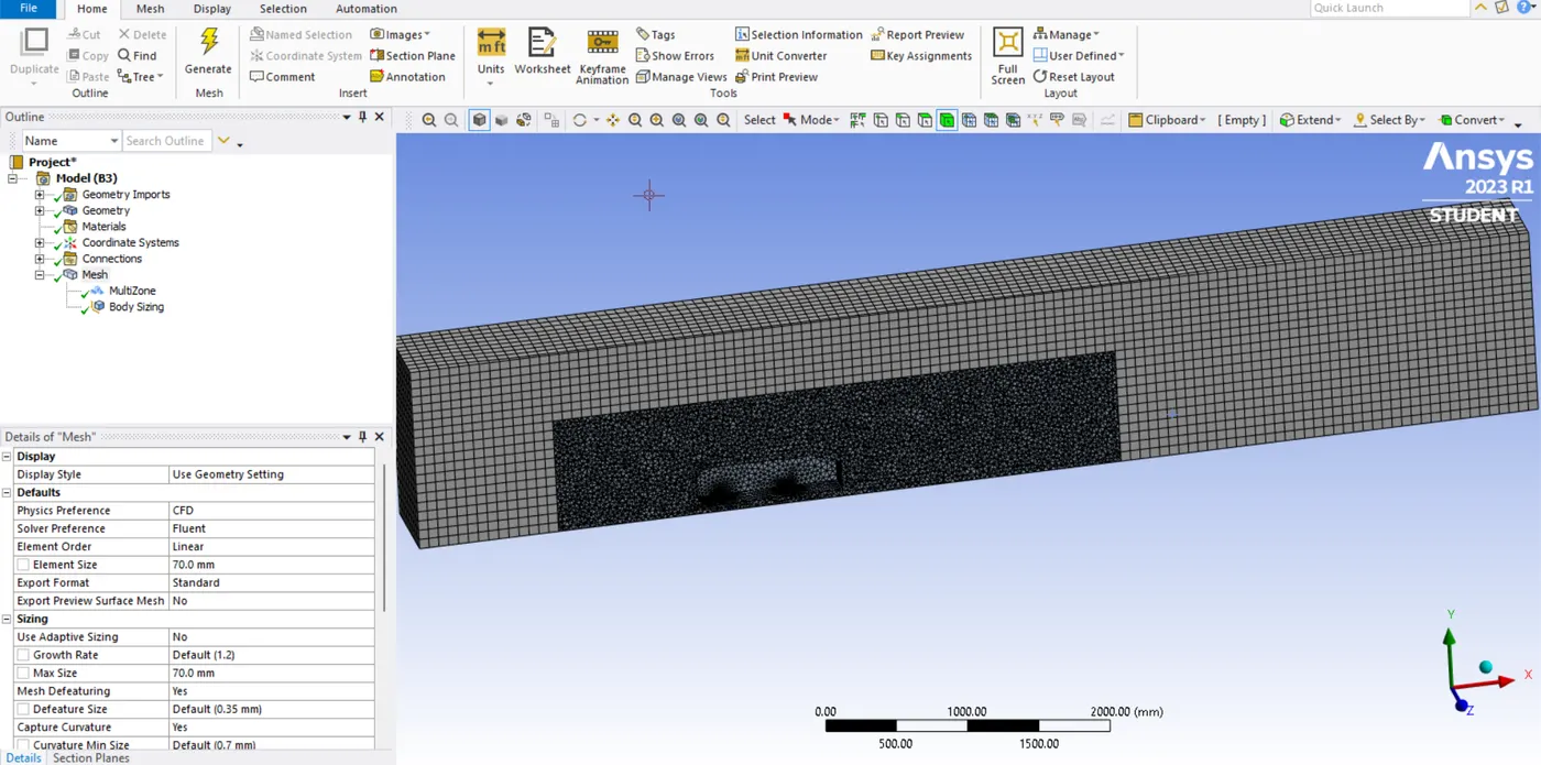
• So, after updating the meshing and now adding the "sizing" underneath the method, we need to make sure that the sizing is more refined and enter the "element size is 50 mm". and then right-click and hit generate the mesh.

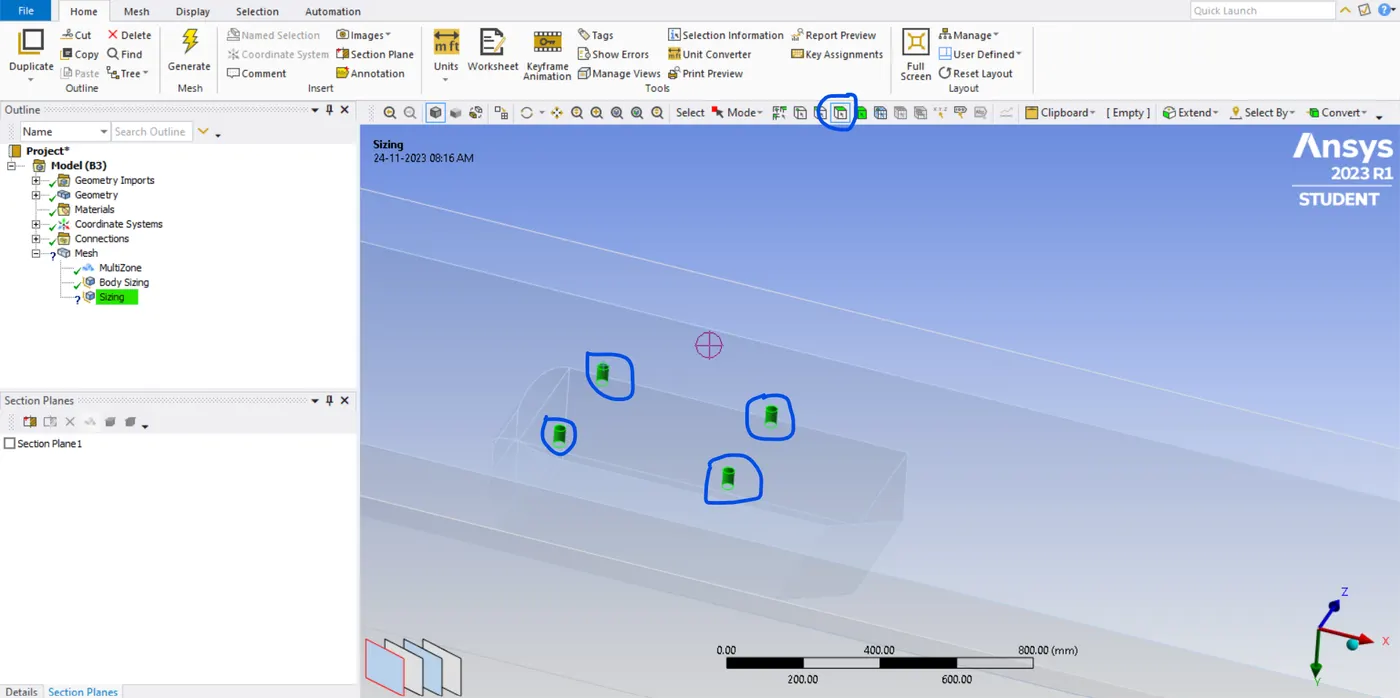
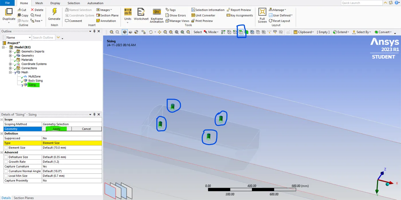
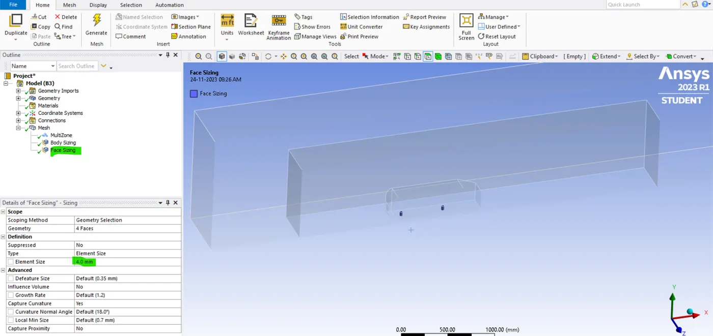
• so, after refining our mesh you can see in our model that in that body the legs or the cylinder face is captured as a polygon. so, here the element size is quite big and we need to refine our cylindrical pillars further. so, to do this add "sizing" underneath the body sizing. so, now we are going to select our entire Ahmed body. so, to do this let's hide all the faces except the Ahmed body, and after that using the "bix selecting" tool select the entire "Ahmed body" and hit "apply" This method is called face sizing.
• so, after that put the "element size is 4mm" and hit generate the mesh. so, now you can see the cylinder area mesh is not captured perfectly so, we need to refine it further. To do this just select the "single selection" tool select the entire cylinder area alone, and right-click to generate the mesh again. so, now the mesh is captured actually.

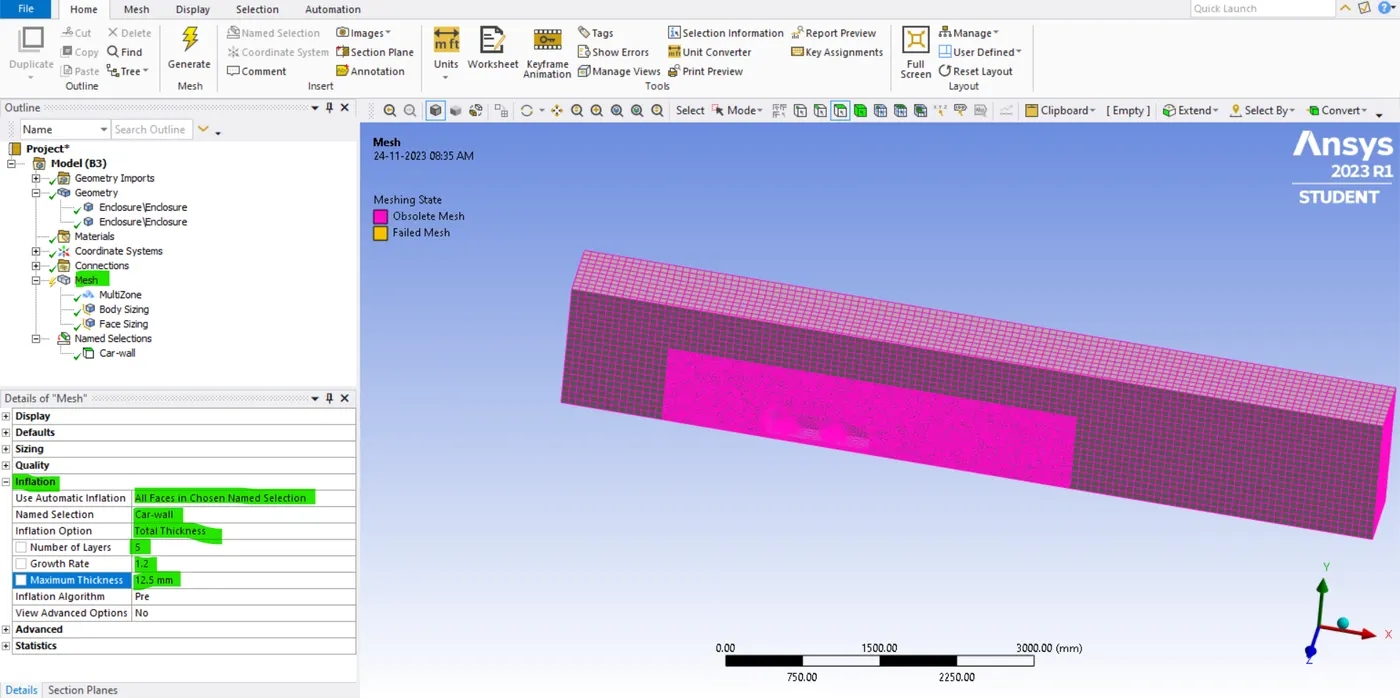
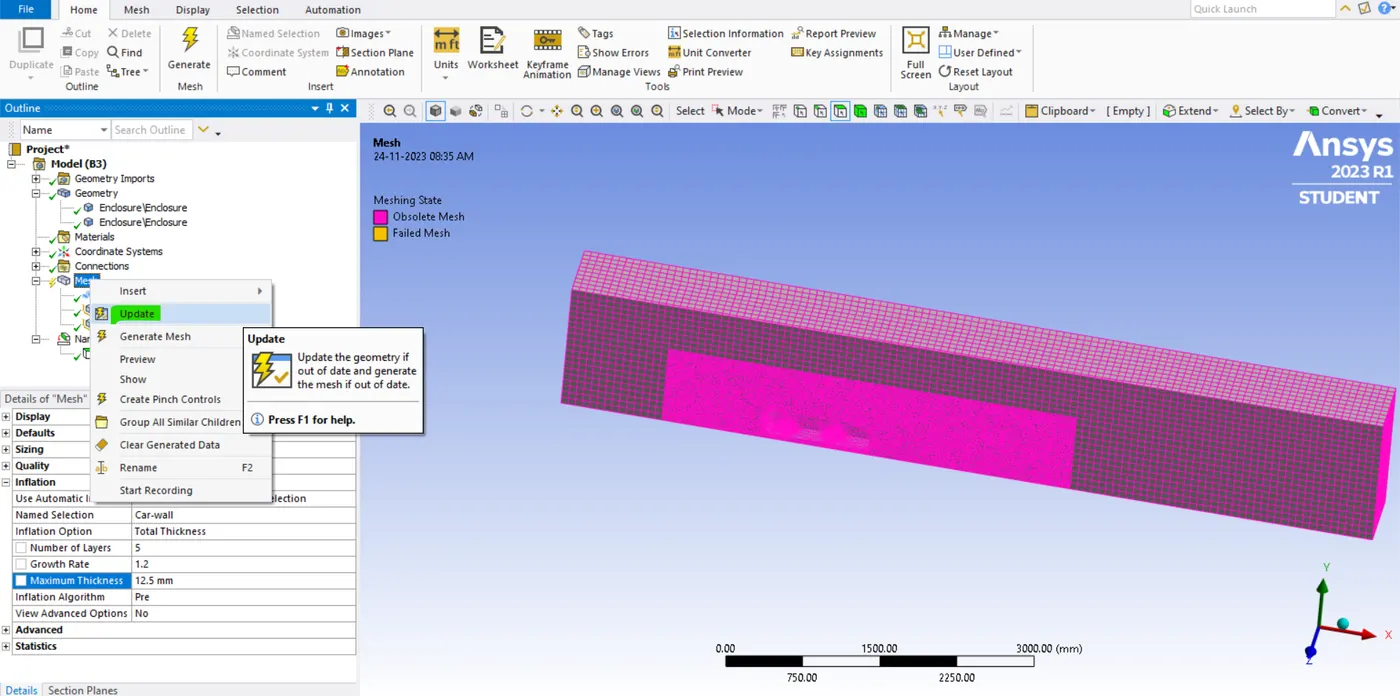
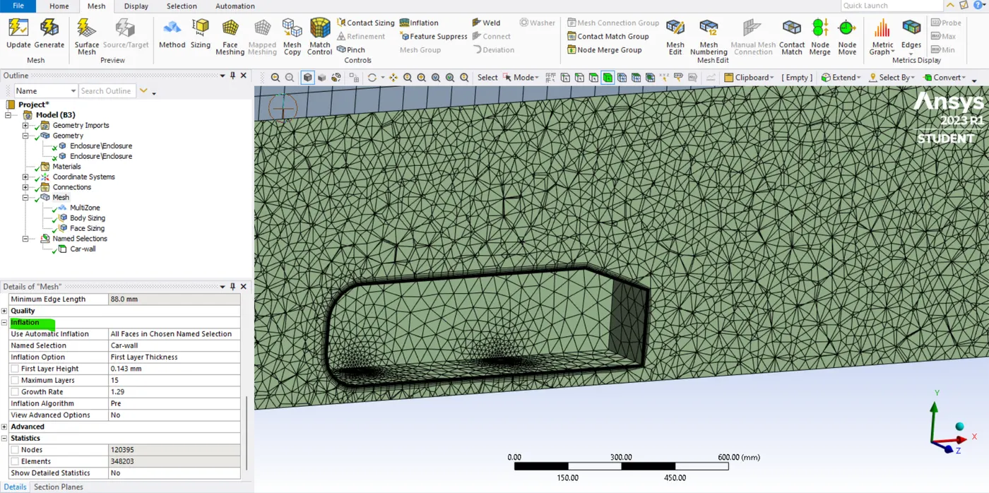
• And now we can also create the bottom layer. so, each cell has different cell centers in different locations and it is not ideal for wall boundary conditions. so, we need to create a set of cells that follow the shape of the surface quite closely.so, these are called inflation layers, to do that right-click on "mesh" and add the "inflation" option.

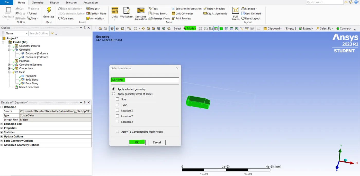
• After adding the option change the inflation type to "all face in chose named selection". and select the Ahmed body and name it a "car-wall". so, after that change the "name section" into "car-wall" and also change the "inflation option" into "first layer thickness". so, this first layer thickness is calculated by our Reynolds number which is the "y+" value, and the max layer value is 15mm. and growth rate is 1.29 and the first layer height is 0.143mm after hit on "generate mesh". so, after that, you can see our inflation layer. it starts small and it keeps growing and the growth rate is 1.29.

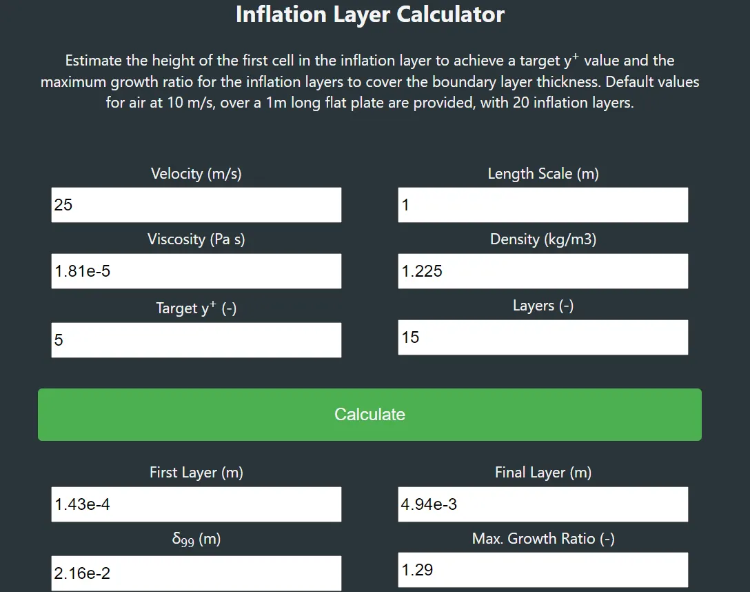
• so, if our first layer thickness is 0.143mm the second is 0.143*1.29, and the third layer is 0.143*1.29^5. so, that says 6.52 mm, and right-click to generate the mesh. so, now our inflation layer mesh looks much more accurate.

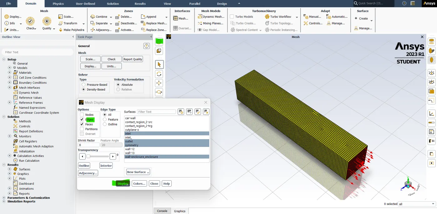
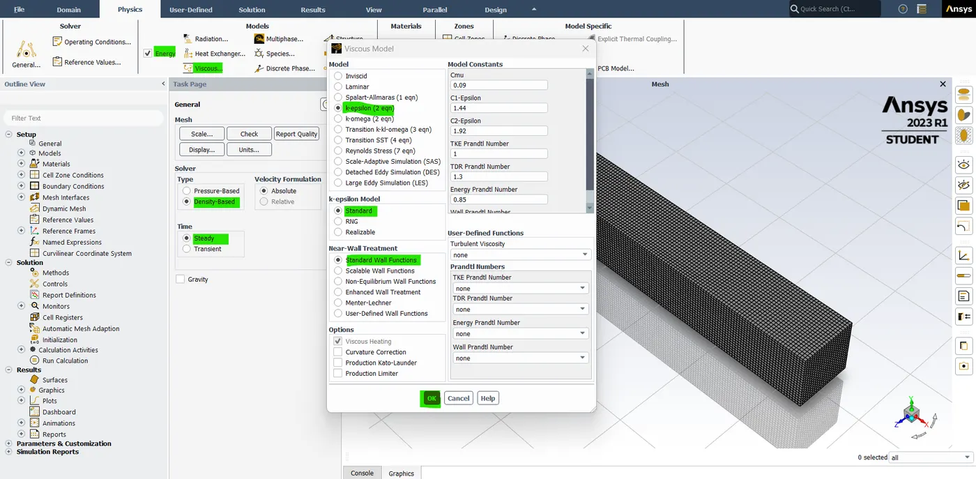
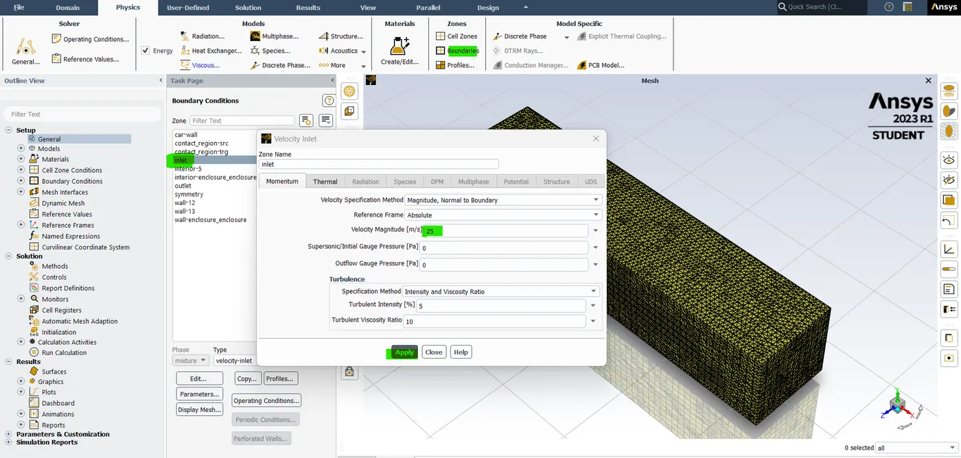
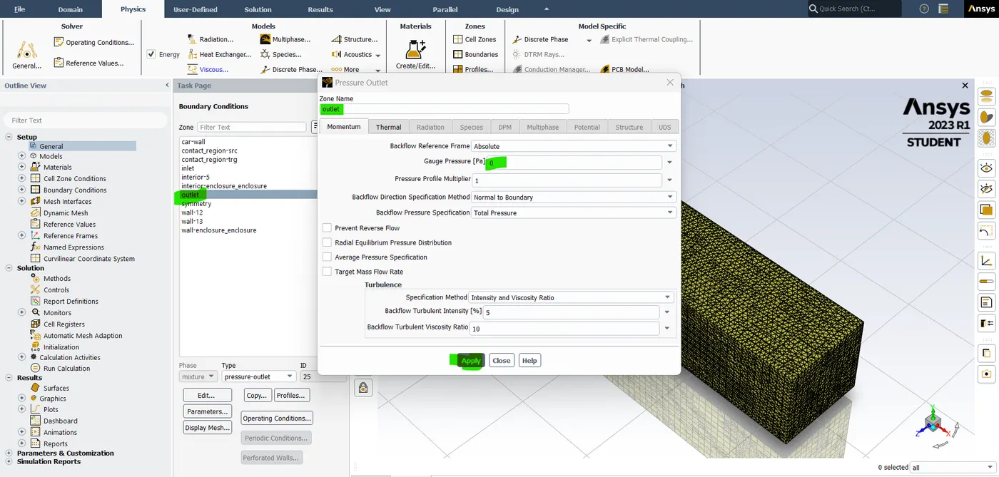
• now close the mesh GUI and update the mesh interface. after that open the setup interface, just go to setting up physics and select the solver type "density-base" solver and the timer is "steady". so, in this case, the inlet velocity is 25 m/s from the mag number point of you it's not a lot from the speed of sound it's just 340. but for convenience assume 300 m/s. In our case, the inlet is going to be 25 m/s. maximum we are looking up the value is 1/6. so basically the max number in this point of you is 0.3 or slightly lower than that. but whenever the max number is 0.3 or above it's good to use density base solver. because we need to take into the good compressibility effects so that's why in this case we are using a "density base solver".
• In this case we are using an energy equation turned on. and the material is air. then let's go to the boundary. and select my inlet type is automatically flagged as a velocity magnitude is 25 m/s and the thermal is 300(k). click "OK".
• And in the time state we can use both the steady state and transient state of the solver. but in this case, we are interested in looking at what's the "Drag force" on the car and what's the "velocity distribution" in the rear end of the car what the wake looks like, and the kind of stuff. so, we are ok with the steady state. so, let's go with that.
• So, we set the physics and in this case, the viscous model is we are using the "turbulence model". so, I'm going to use the "k-epsilon" and that's going to be the initial choice of turbulence model and this is not a good one for this model. but are just using after that click "OK".

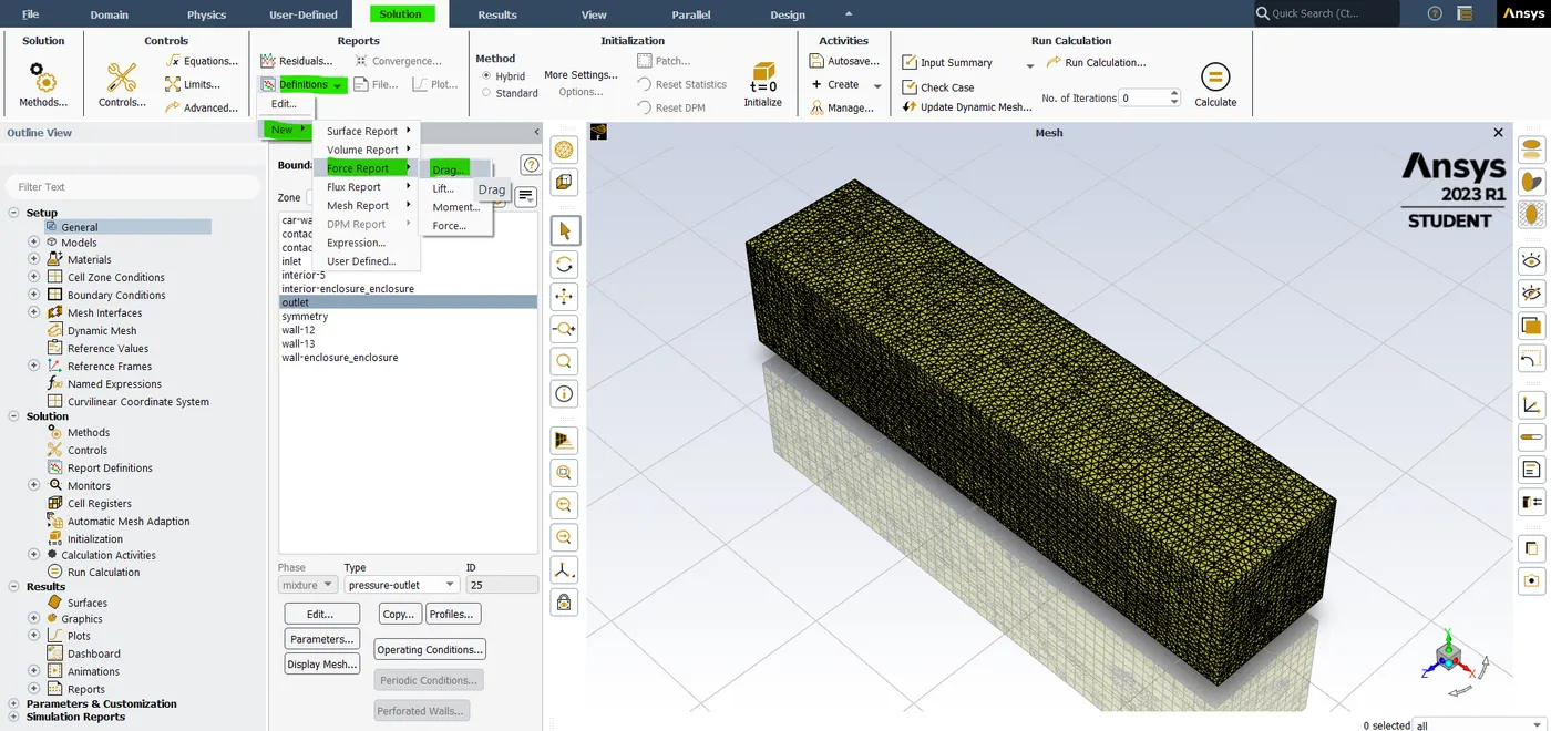
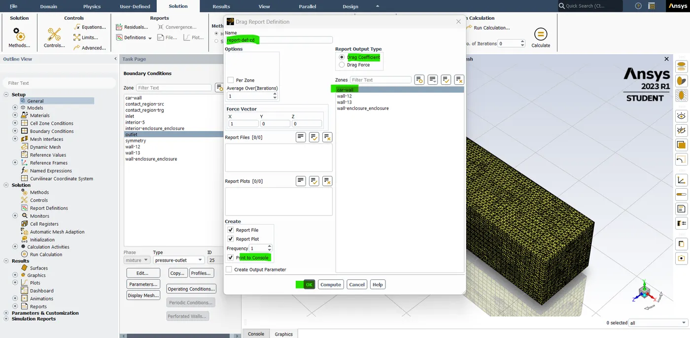
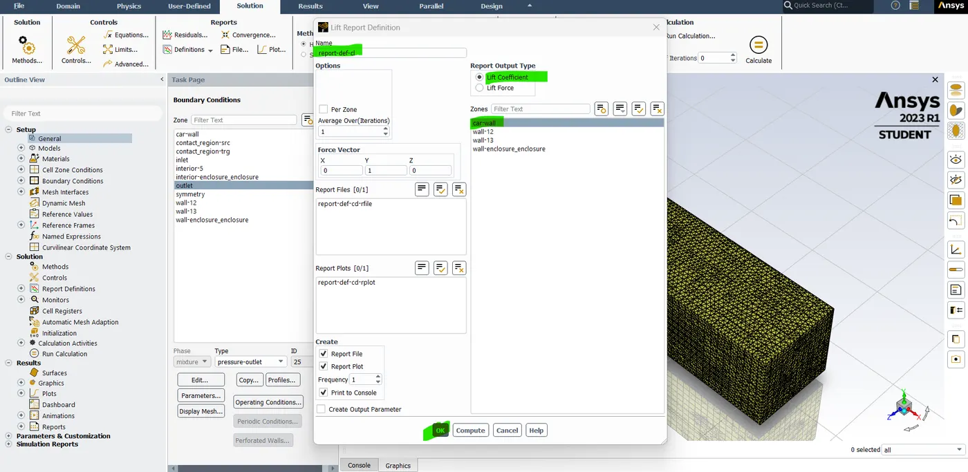
• So, in this challenge we are looking for a "Drag co-efficient" so, To do that we need to go into solutions -> Definitions -> Force Report -> now select "Drag Force". In that select drag coefficient and car-wall and then hit on "ok".
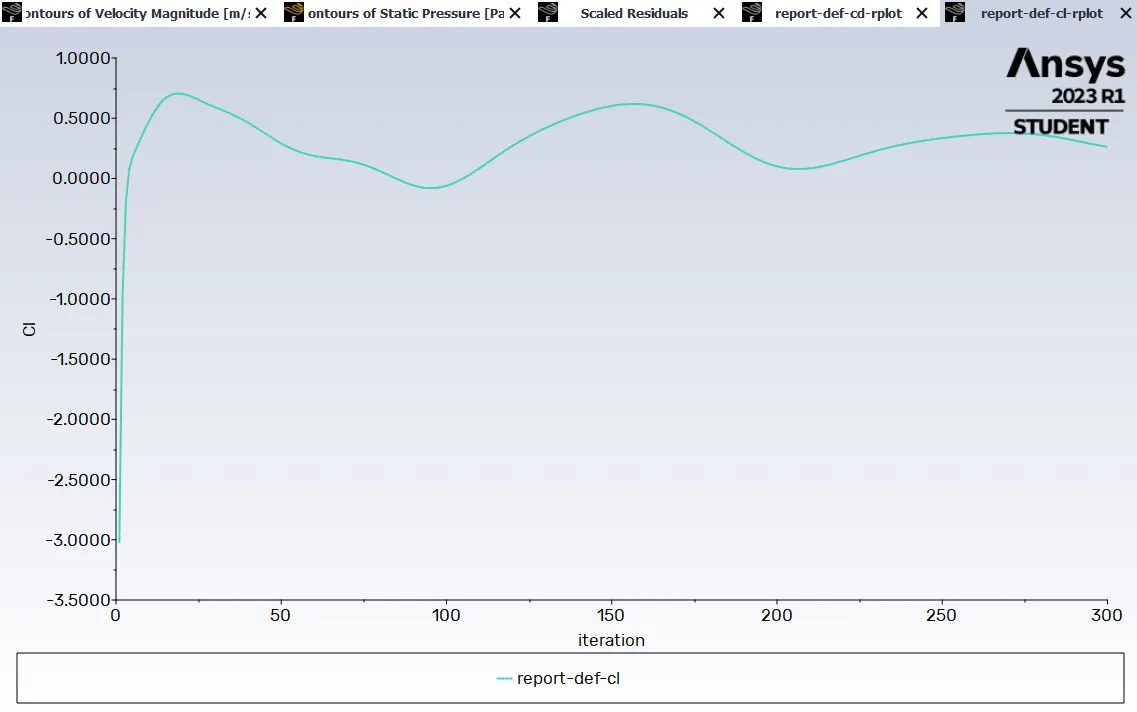
• Similarly repeat the processes for "Life coefficient" and hit on "ok".

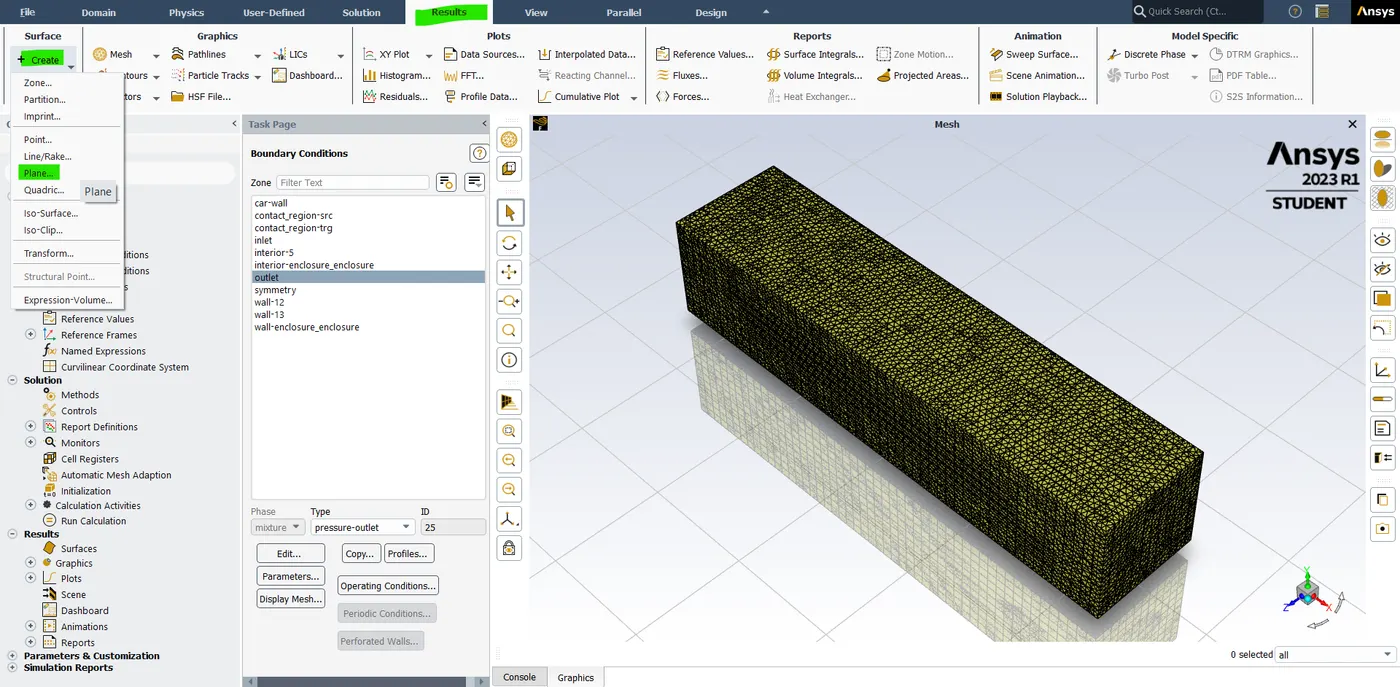
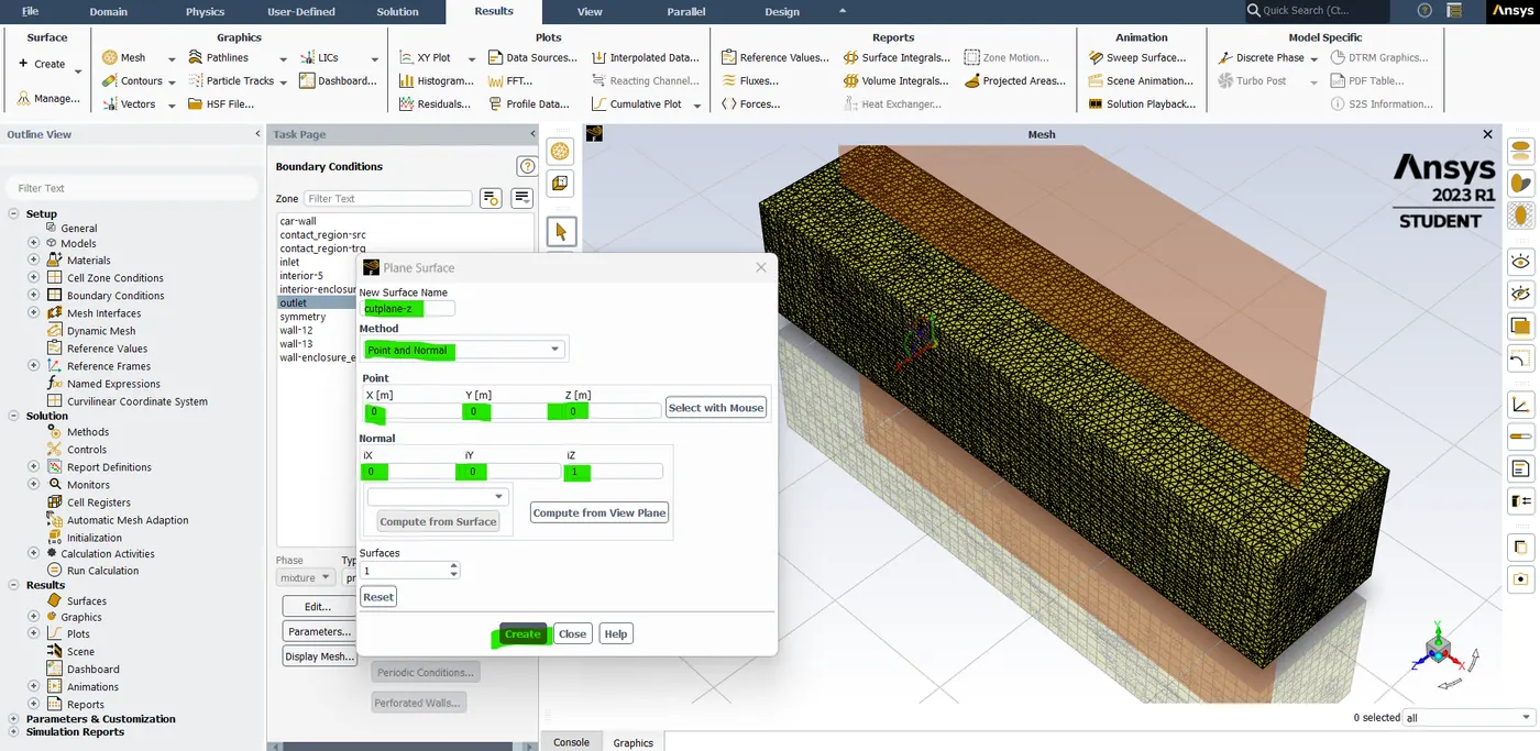
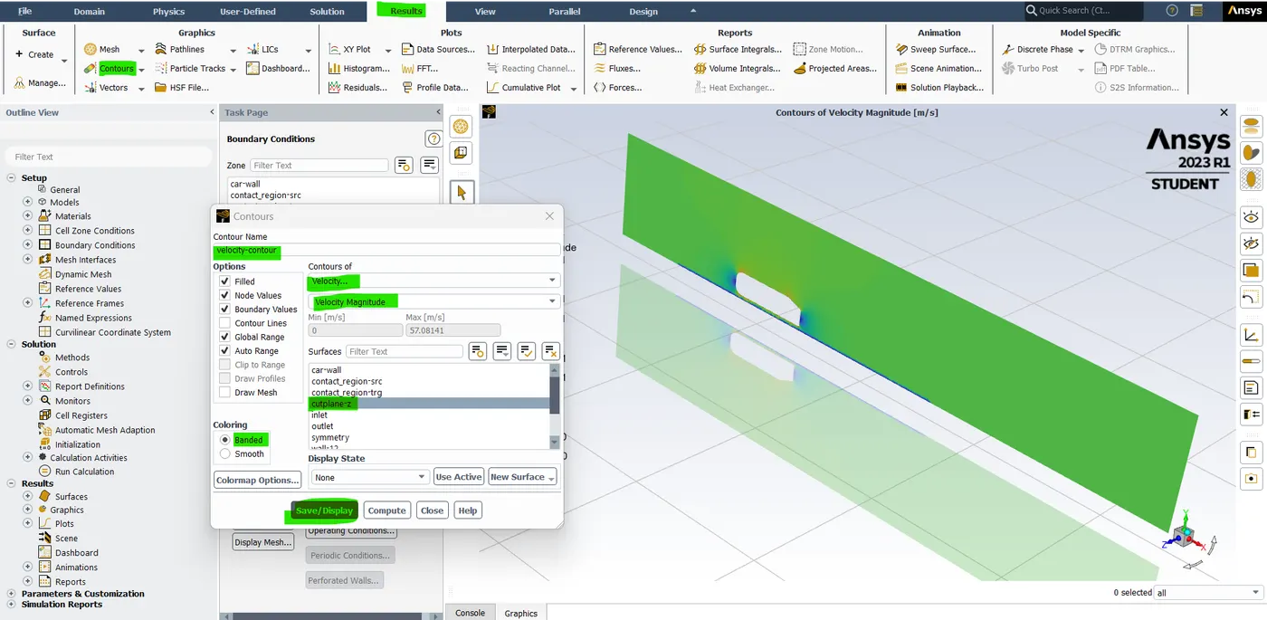
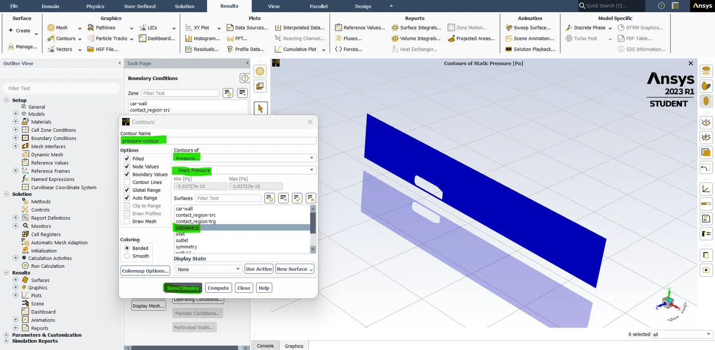
• Now we need to monitor the amount of velocity and pressure applied on the body. so, to do that we need to go into Results -> create -> plane. so, in that plane select the method as point and normal. and the points are XYZ- axis is 0 and the normal is ix, iy-axis is 0, iz-axis is 1. and named as a "cut plane-z".
• now we need to create a contour plot for velocity and pressure to monitor the amount of velocity and pressure applied to the body. so to do that we need to follow the steps in the above image.

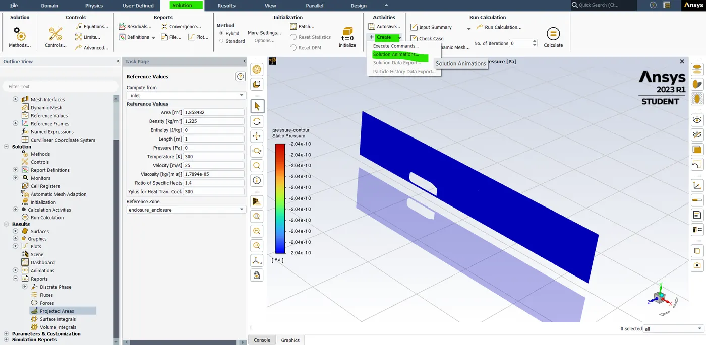
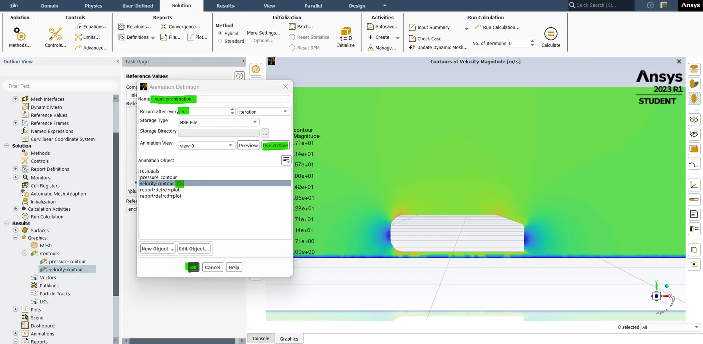
• so, now we record this simulation as an animation video. for that go into the solution section -> create -> select "solution animation". In that named as a "velocity-animation" enter the iteration is 5 and select the "velocity contour" set the view and hit use active and then hit on "ok".
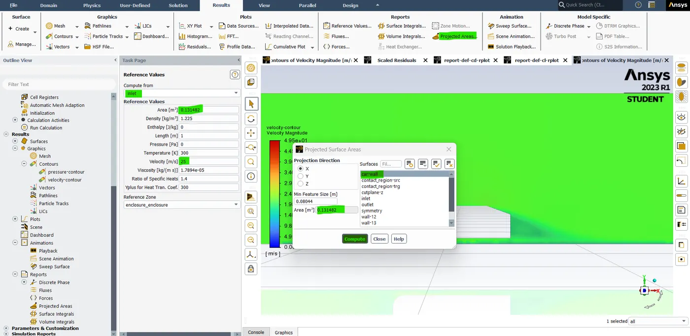
• Now before simulating this challenge we need to set the reference value of the inlet. so go to the reference value and select the inlet and the Area is 0.131482. To get this area value go to the Result section select the projected area in that select car-wall and hit "compute" Now we have the inlet area of the car wall just copy that value and apply it to the reference value.
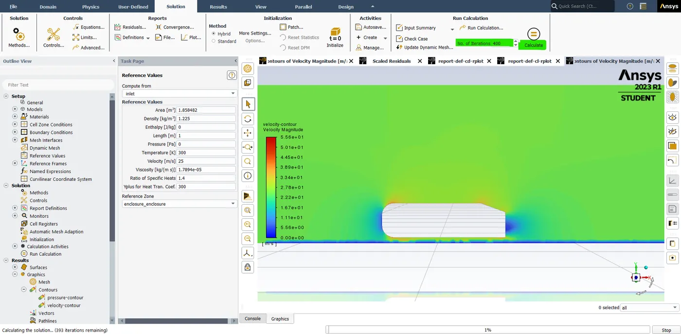
• Now to run this simulation enter 400 into no.of.iterations and then hit "Calculate".

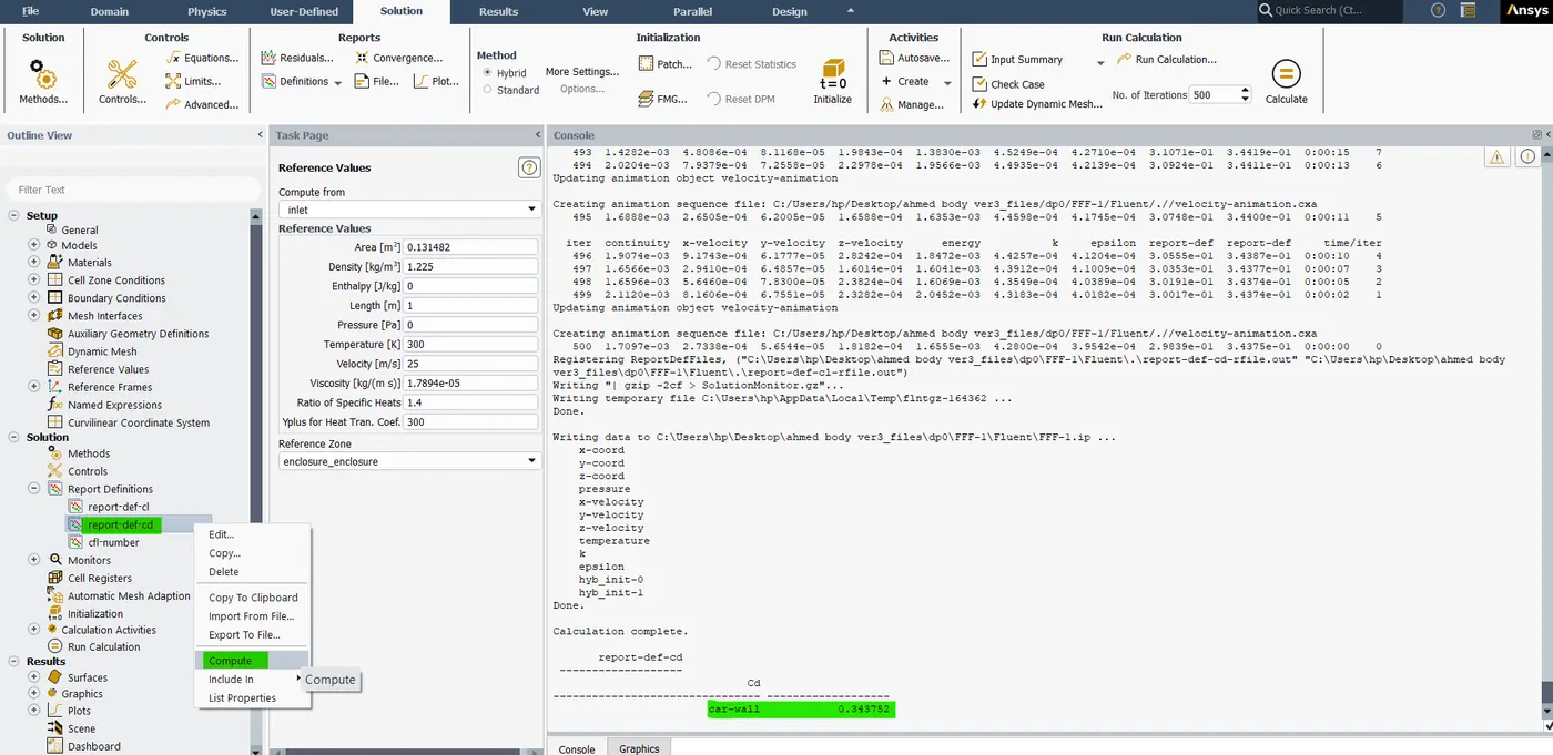
• Once the simulation is done just go to the solutions -> report definitions -> select the "report definition_cd" and right-click on that hit compute. Now we have the Drag coefficient (CD) of 0.343752. so, this value is way more accurate. After that close this meshing GUI and then go to the post-processing section which is open the Result GUI.

RESULT:-

Drag plot:

Lift plot:

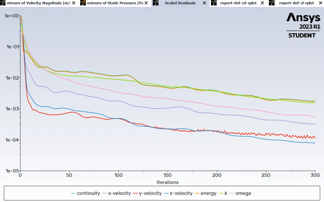
Residual plot:

Velocity Contour:

Pressure Contour:

Vector plot:

With Split Body Command(with mesh element size as 100 mm and 50 mm):

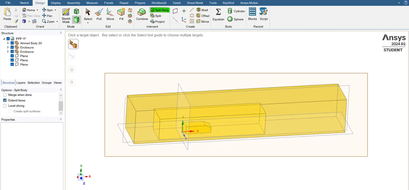
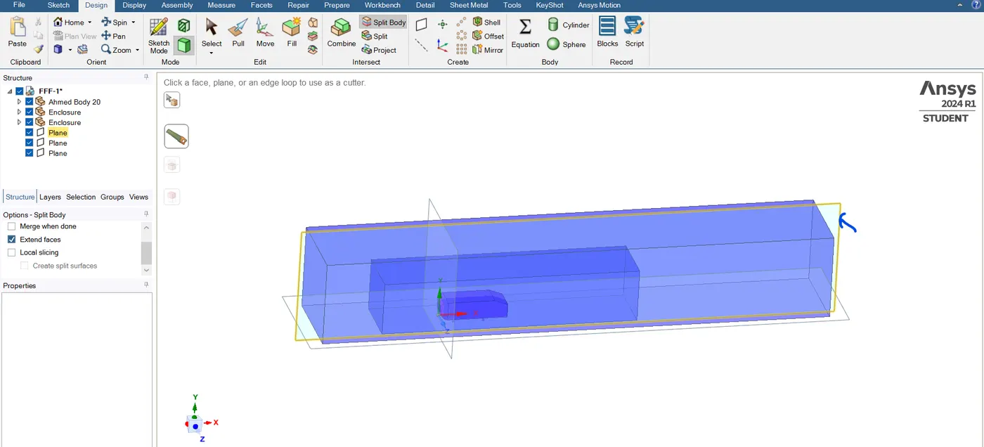
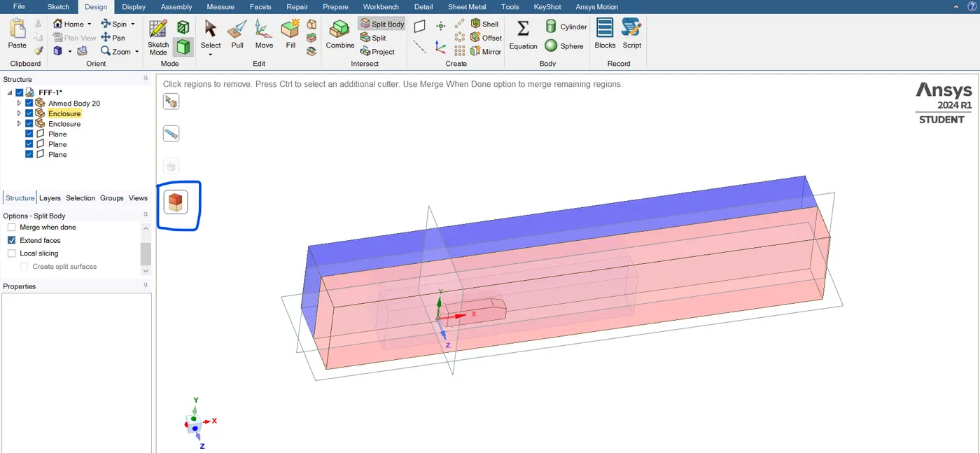
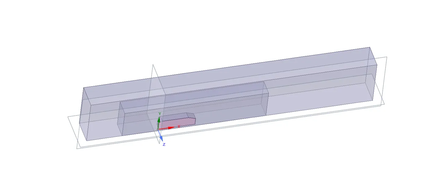
• So as per the challenge guidelines we need to cut this geomentry into symmetrically. So, to do that we need to use the "Split body command" option. so first go to the Design section and then click the "Split body" command and then drag select the model entirely and then click the "x-direction plane". so now the plane is projected on the body.
• now we need to select that box tool to delete the other half. To do that first select the box icon and click one by one on the model till the Ahmed body.
• so, after that, the other half has been cuted. now we can perform the next part of the simulation.

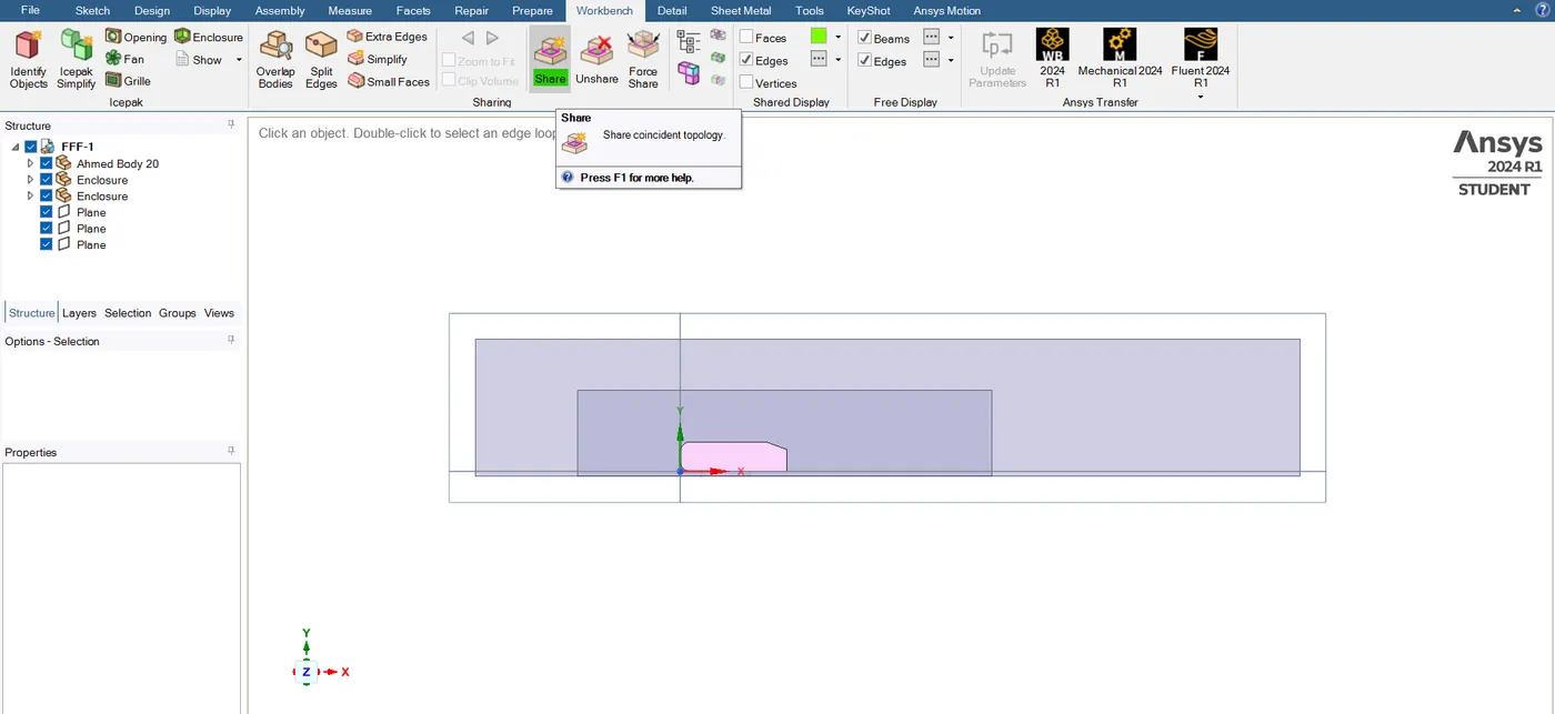
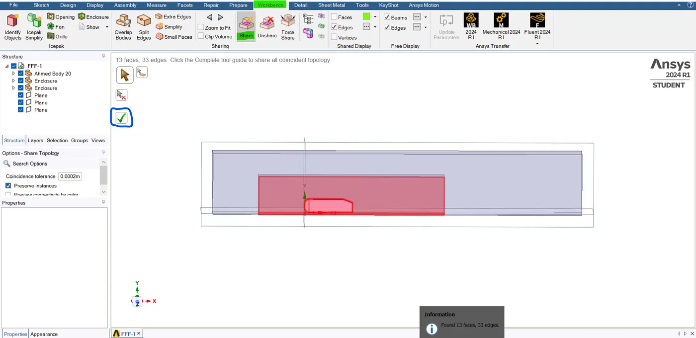
• The Ahmed body has two enclosers when we are meshing this body we need to enable the share Topology option so that the information can flow from the inner encloser to the outer encloser through the grid connection.
• To enable the "share topology" option, first go to the workbench section and then select the "share" option, it's automatically identified and it selects the encloser connecting with others. now just click that "Tic mark" and it'll be automatically enabled.

• The above image is a "Share-Topology" enabled version. Now the Grids are connected with each other encloser.

Grid Independence Test:

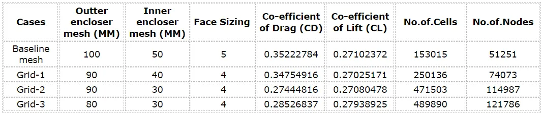
• To choose the correct mesh element size, grid independence is the perfect choice for choosing the different mesh element sizes for running the simulation. The mesh element size gives the accurate value for the coefficient of Drag and it takes less computational time to optimize the mesh element size for this model.
• The above and the following results are obtained for the combination of different mesh sizes. The maximum cell count that I used here in the academic version of the fluent is 512000 cells. The flow is taken as air and its properties which flow at the value of 25 m/s.
• So, there are notable changes in the three cases, mesh is more refined from the baseline mesh and grid 1 & 2 to check the grid dependency. a smoother mesh provides an accurate mesh result. From all three cases, we can conclude that the flow is more refined at lower element sizes.
• The coefficient of drag attains a consistent value up to the 2nd decimal place grid-2 and grid-3. the grid-3 holds the maximum refinement and the cell count is close to the maximum value. The error rate of the drag coefficient obtained in Grid-3 is [23.48%]. The error rate produced in Grid-2 is [28.35]%. Hence grid 2 and grid 3 both produce the close value and both mesh results are considered mesh independent.
• Error rate Formula :- (Baseline mesh_CD - Grid-2_CD / Grid-2_CD ) x 100.

Baseline mesh:

Grid-1:

Grid-2:

Grid-3:

Q&A:

Q1. Describe Ahmed's body and its importance.

Ahmed's body is a simplified car model that is created mainly because of comparing and so validating the computational simulation result with the experimental results to check whether the simulation result is correct. Ahmd body is a generic car model first proposed in Ahmed 1984. All ground vehicles can be termed bluff bodies. so we can perform the external flow analysis computationally simulation to reduce the drag force on the car by capturing the wake region formed behind the car surface. The analyzed body can capture the essential feature of the flow that characterizes the modern car.

Ahmed's body has a slant rear end whose angle can be manipulated and the corresponding drag and lift can be calculated. The Ahmed body portrays how to calculate the turbulence flow field around a simple car-like geomentry using a turbulence flow K-epsilon interface.

Q2. Explain the reason for the negative pressure in the wake region.

The wake region is re-circulating the flow immediately to the moving or stationary solids body. This is caused due to the flow of the fluid around the body. so, the wake region is the region where the velocity gets decreased because of sudden blunt geomentry change behind the Ahmed body. The airflow from the surface will cause higher resistive force and higher velocity gradient compared to airflow far away from the surface. so Thus, the air flowing away from the surface will tend to keep the air flowing with higher velocity. This is due to the velocity difference of the fluid (air). Thus, there is a pressure difference that occurs behind the Ahmed body due to the pressure difference from the high-pressure region to the low-pressure region. So, that is why the causes of Negative pressure in the wake region.

Q3. Explain the significance of the point of separation.

The separation point is the point where the air stops sticking to an object that is moving through the air. So, when the object is moving along with the air, the air molecules push back on it and it resists the object's movement. so, this resistive force is called pressure drag force on the Ahmed body as pressure flows from the high-pressure region to the low-pressure region.

CONCLUSION:

The flow over Ahmed's body is simulated and the wake region is also visualized with the help of vector plots and contour plots and it has been analyzed. The drag co-efficient and lift co-efficient are also estimated. the importance of the Ahmed body the reason for the negative pressure in the wake region and the point of separation are also discussed. Finally, the gird independent test is also conducted successfully.