Week 3 - External flow simulation over an Ahmed body.
The aim of this challenge is to run an external flow simulation over an Ahmed body, first with a base line simulation and then with a more refined set-up with a finer mesh and inflation layers based on the inputs gathered from the base-line run. The effect that a finer mesh has on the results are also studied via a grid independance test.
Q)Describe Ahmed's Body and its importance.
An Ahmed Body is a standardised bluff body geometry that is used for validating CFD data.
A bluff body is a body that has separated flow over a substantial part of its surface (by virtue of its shape). It can alternately be defined as a body whose surfaces are not aligned with the streamlines in a flow.
The basic dimensions of this standardised body as proposed by S.R Ahmed in 1984 is shown:
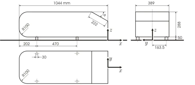
(All dimensions in mm.)
The geometry is simple enough for accurate flow simulation without losing any of the practical features that is relevant for automobile design and engineering. The Ahmed body is thus a benchmark for many aerodynamic simulation tools as the data from wind tunnel simulations of the Ahmed body is widely available.
Q)Explain the reason for the negative pressure in the wake region.
Negative pressure simply implies pressure less than the atmospheric pressure.
The wake region following the rear of the car is characterised by a low-pressure turbulent region caused by the separation of fluid over the Ahmed body owing to its bluff geometry. The fluid which is behind the wake region (at atmospheric pressure) tries to fill in this low-pressure region. As this fluid column is dragged in, it creates vorticity. The slant angle of the rear of the Ahmed body plays a major role in this phenomenon.
Q)Explain the significance of the point of separation.
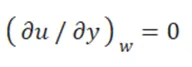
The point of separation is where the fluid stops sticking to the wall surface. In more technical terms, it marks the point of detachment of the boundary layer of fluid flow from the wall surface resulting in vortex formations and thus the formation of turbulence.
For two-dimensional steady flows, it is defined as the point where the wall shear stress becomes zero.
Base line simulation set-up:
A base line simulation was first set up with no forms of mesh refinement.
This was done so that the wake region could be estimated so that the region where the mesh refinement had to be done could be effectively estimated.
The given model was put in an “enclosure” with the instructed dimensions. This option was present in the ‘Prepare’ tab in the ‘Analysis’ group when the model was edited in SpaceClaim.
The next step was to split the model into two, making use of the Ahmed body’s symmetrical geometry. Only one of the split bodies could thus be used for further simulations.
For this, a plane in the middle of the enclosure with its normal along the z-direction was created (the model is aligned lengthwise in the z-direction. The model is split along this created plane using the ‘Split Body’ option in the ‘Intersect’ group in the ‘Design’ tab.
Of the split bodies, one was deleted.
After this, the model was meshed without any inputs for refinements as this was just for a base-line simulation.
The simulation was then set-up.
Velocity of 25m/s translates to 0.075 Mach at 300K (taking the speed of sound at 300K to be around 332m/s),
Thus, we can ignore compressibility effect of the fluid and thus the ‘Pressure-Based’ solver can be used.
For the viscous turbulence model, the k-omega model was chosen as it is more apt for low Reynolds number flows. Also, for analysing the drag and the lift, we need to analyse the laminar sub layer of the boundary layer of the flow that is the closest to the wall. The ‘Steady’ state solver was selected. In the ‘Materials’ section, air was selected. Also, the ‘Energy’ box was checked.
In the ‘Boundaries’ section in the ‘Zones’ group, the inlet velocity was set to be 25m/s and the temperature was set to 300k.
From the ‘Results’ tab, ‘Surfaces’ group, a velocity contour was created along the length of the model (normal along the z-direction).
The solution was then initialised (hybrid initialisation) and solved for 500 iterations.
In post processing, two lines were constructed along the height of the wind tunnel located at “x=2m” and “x=3m” (behind the Ahmed Body).
The data ‘Cut’ from these lines were then expressed on a chart.
The y-axis showed the ‘u’ component of velocity and the x-axis showed the vertical space coordinates.
Results from the base-line simulation run:
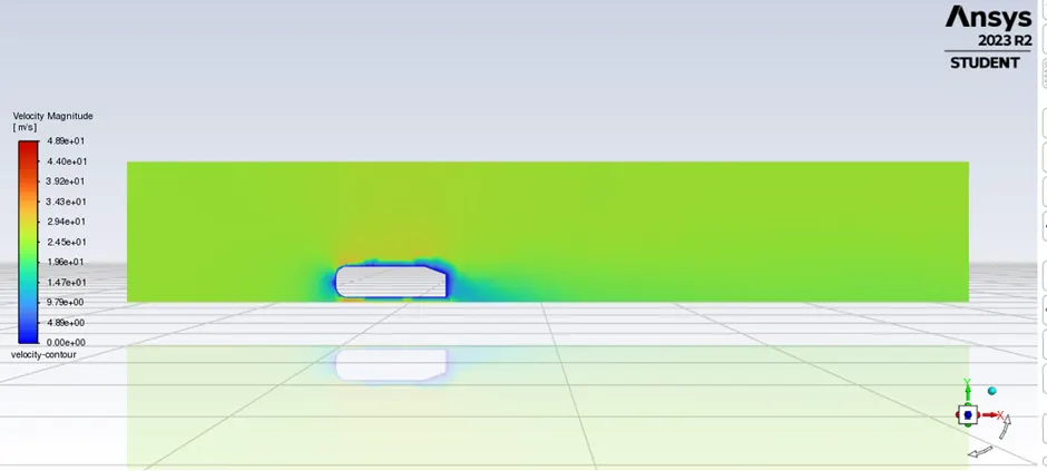
(velocity contour; coarse mesh.)
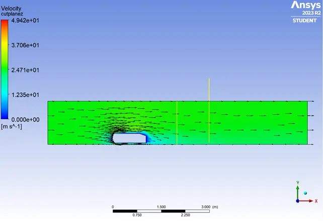
(With vector plots.)
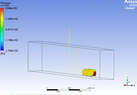
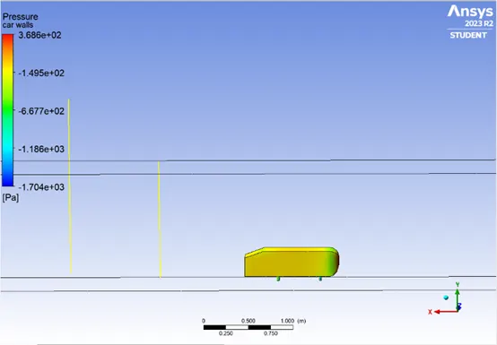
(Pressure plots.)
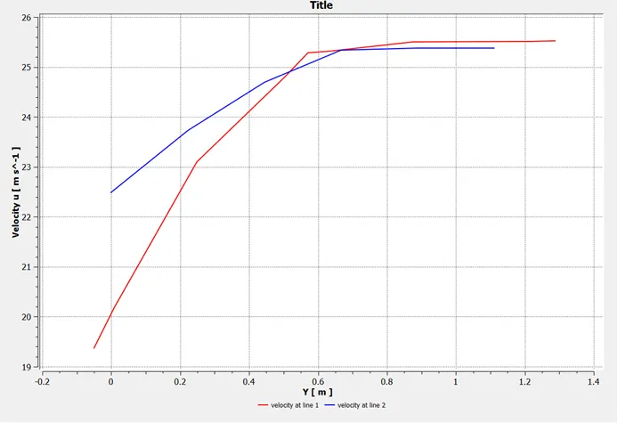
(Velocities at lines 1 and 2.)
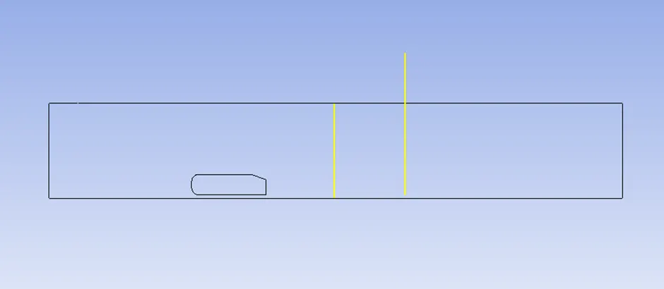
(Positioning of lines 1 and 2 respectively.)
With mesh refinement:
Refined mesh:
With an estimate of the wake region (with the help of the coarser mesh from the base line run),
An enclosure was made inside the existing one such that the wake region would be enclosed in it. The finer mesh can be confined within this region. This eases the load on the computational capabilities and is thus an effective method.
The region trailing the Ahmed body (where the wake region lies) was made to be 1.2m long.
With this enclosure made, the meshing module was then opened.
The faces were duly grouped into their named selections. The walls were named “symmetry-walls”,
The walls of the Ahmed body were named “car-walls” and the inlet and outlet were named accordingly.
The mesh size is inputted to be 0.1m. Then the body between the first enclosure and the smaller enclosure made was meshed with the “Hexa” type mesh by creating a ‘MultiZone’ meshing method for this region. This was done because the geometry is simple and ‘Perfect’ (that is, it lacks complex features and is made up of box like structures).
A ‘Body Sizing’ method is used for the space between the smaller enclosure and the Ahmed body.
The element size is inputted to be 0.05m.
In order to study the drag and the lift forces, the physics of the viscous sublayer would have to be analysed. Thus, the value of ‘y+’ (dimensionless wall coordinate to study the boundary layer) was taken to be 5 so that the laminar sub layer of the boundary layer closest to the wall would be taken into account.
With the help of a ‘y+’ calculator, the value of the first layer thickness for the boundary latyer and the appropriate growth layer for 18 layers was calculated.
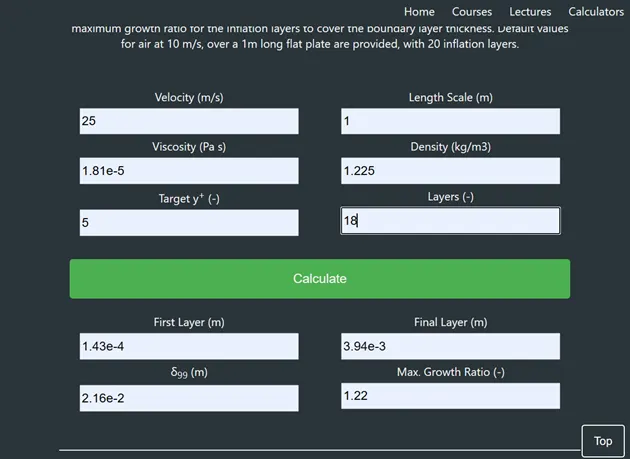
These values were inputted in the ‘Inflation’; sub-menu.
The mesh was then generated.
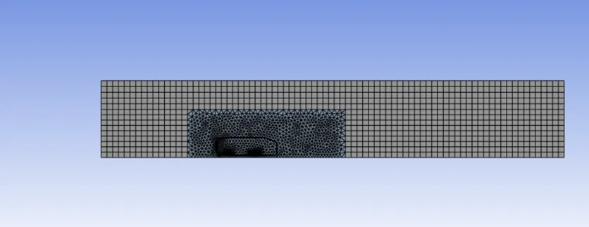
The physics was set up in the same manner for the base layer.
The results obtained were:
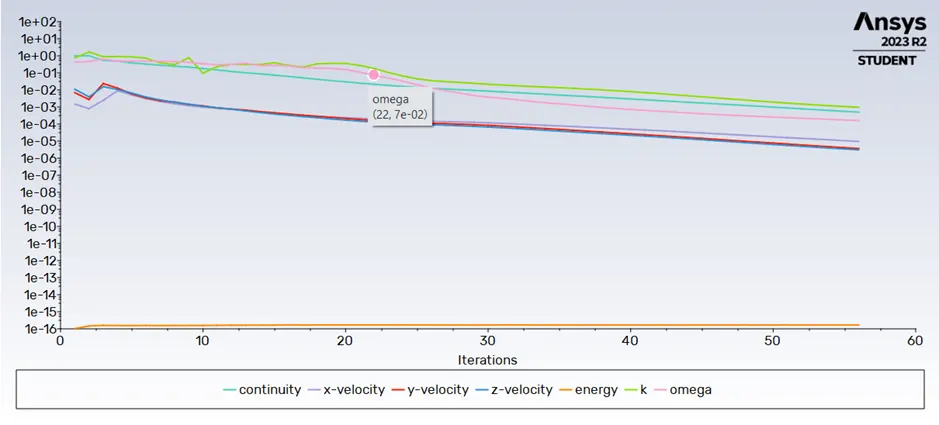
(Scaled Residuals.)
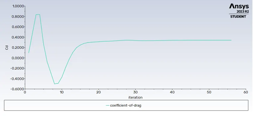
(Plot for coefficient of drag)
The computed value of coefficient of drag was: 0.34055942.
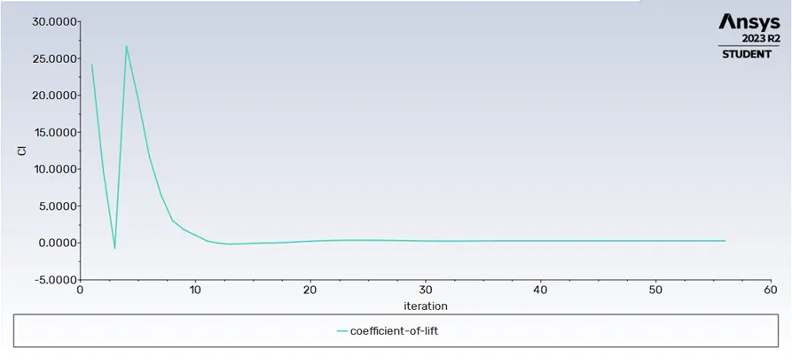
(Plot for coefficient of lift)
The computed value for the coefficient of lift was: 0.28416167.
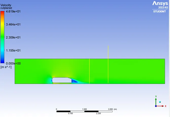
(Velocity contour.)
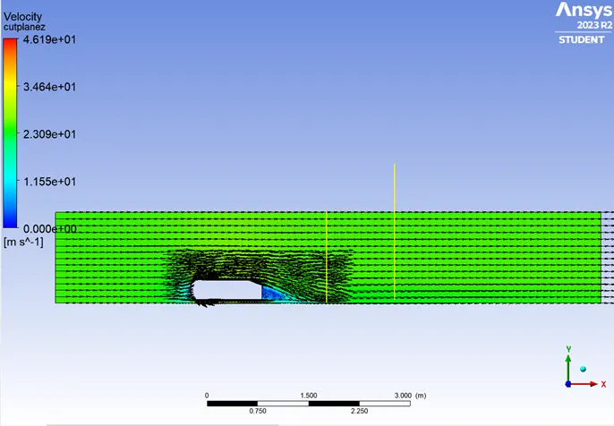
(With vector plots.)
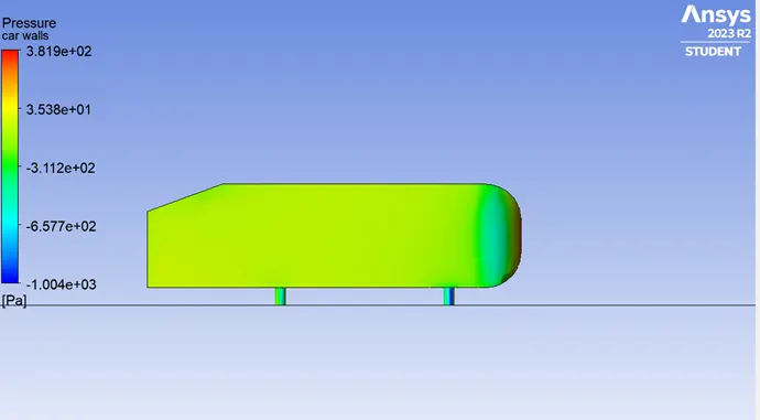
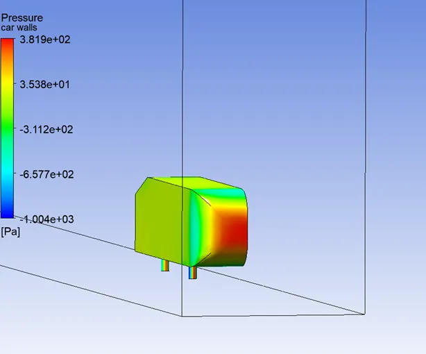
(Pressure contour.)
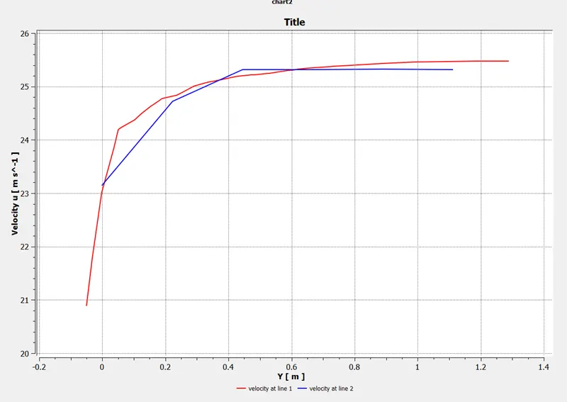
(The data from lines 1,2)
Refining the mesh further for grid independency test.
With the current inputs, the number of elements were 129780.
The element size was changed to 0.08m and the size in the smaller enclosure (the region for refined mesh) was changed to 0.03m.
This caused a jump in the number of elements to 343447.
Further refinements were thus made to the smaller enclosure only.
Obtained results:
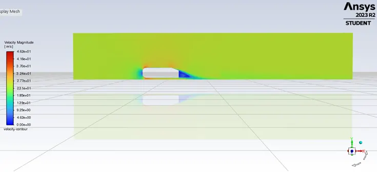
(Velocity contour.)
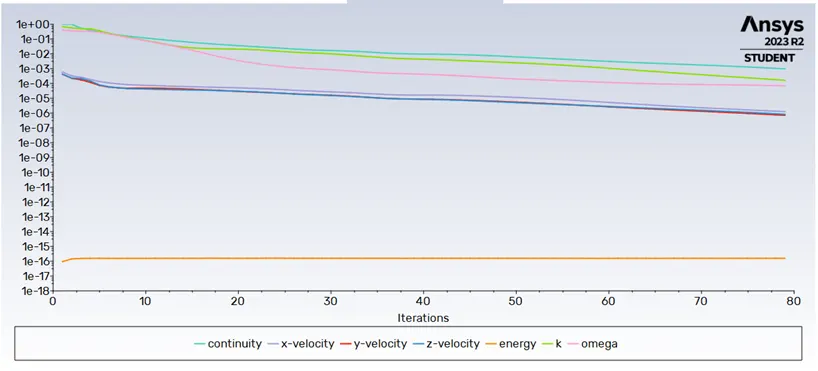
(Scaled Residuals.)
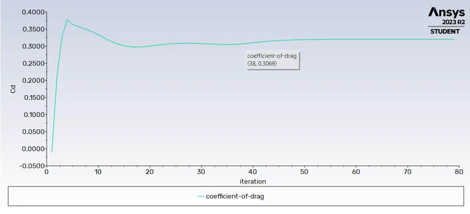
(Coefficient of drag)
The computed value of coefficient of drag: 0.32025468.
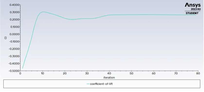
(Coefficient of lift)
Computed value of coefficient of lift: 0.26143605.
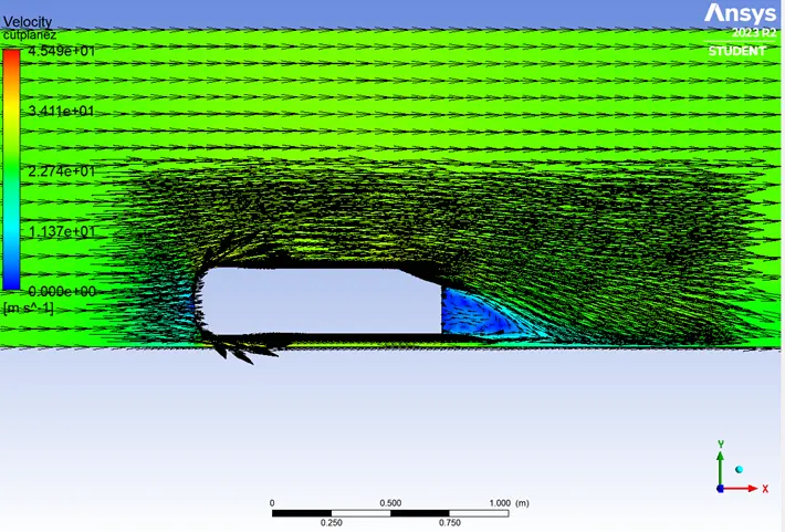
(Velocity contour with vector plots.)
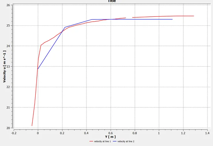
(Velocities at lines 1 and 2.)
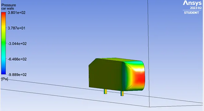
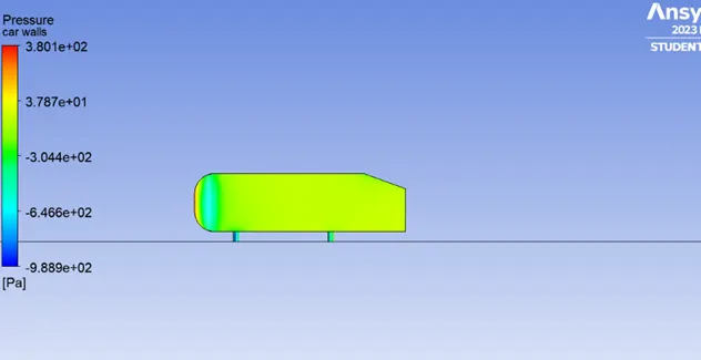
(Pressure contours)
Now, the mesh inside the inner enclosure was further refined by reducing the size to 0.025m.
The number of elements jumped to 530932.
The results: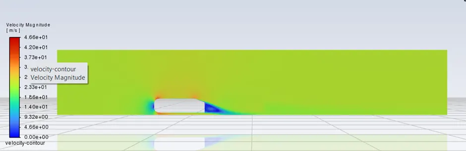
(Velocity contours.)
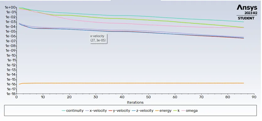
(Scaled residuals.)
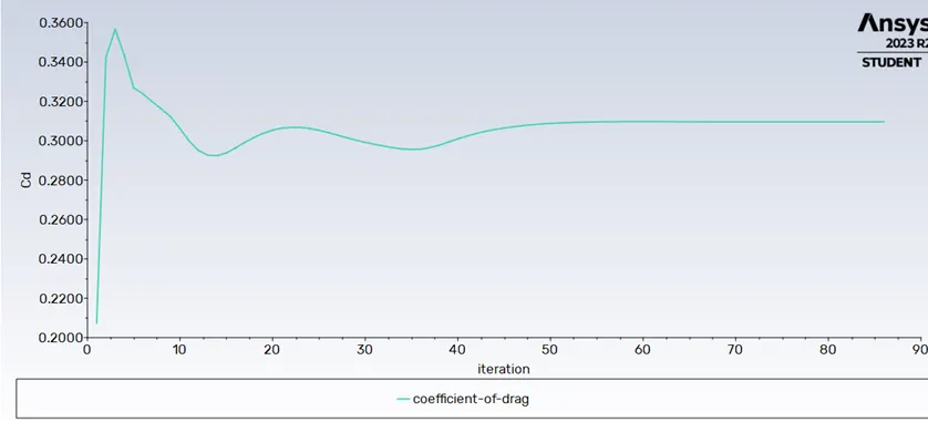
(Coefficient of drag.)
The computed value of coefficient of drag: 0.30962785.
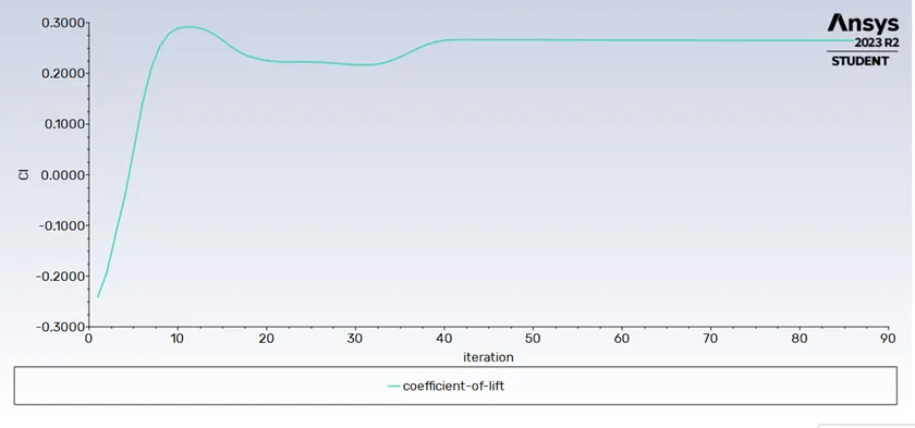
The computed value fi coefficient of lift: 0.26480106.
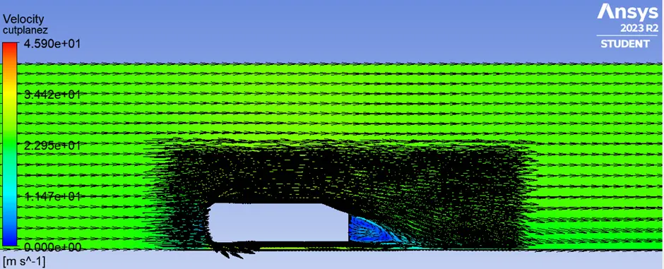
(Velocity contour with vector plots.)
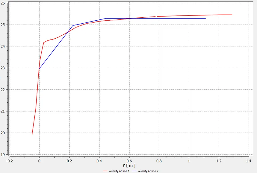
(Velocities at lines 1 and 2.)
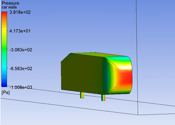
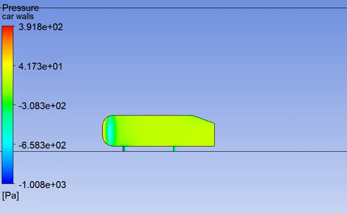
(Pressure contours.)
Observations and learnings:
This challenge helped in understanding the real world industry relevance of the Ahmed body.
This challenge also helped in understanding the mesh refining tactics used in industries.
The importance of inflation layers were understood in the analysis of parameters like drag forces and lift forces that are very sensitive to the boundary layer thickness. This helped me understand the real-life applications of the boundary layer theory.The effects of mesh refinement on the results were also studied. The most observable difference was in the velocity contour plots with vector plots. The finer the mesh, the more sharply defined the wake region was. This was also characterised by the larger number of vector lines defining the flow. In comparison to the finer mesh, the simulation run on the base-line mesh produced results that were a lot more diffused due to the coarser nature of the mesh. The vector plots for the velocity was also much more sparse in comparison to the simulations set up with finer meshing.