Week 3 - External flow simulation over an Ahmed body.

AIM:

Simulate the flow over a Ahmed body with default air properties moving at 25 m/s.

OBJECTIVE:

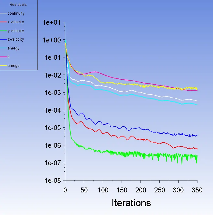
1. To check the convergence of flow.
2. Plots of coefficients of drag and lift.
3. To check grid dependence and select refined mesh for analysis.
4. Calculate drag and lift coefficient (For velocity of 25m/sec, the drag coefficient should be around 0.33)
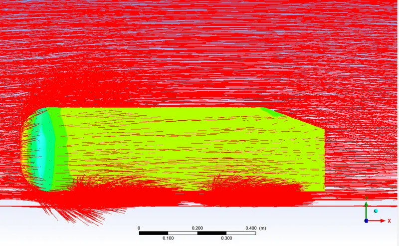
5. Show velocity vector in wake region.

INTRODUCTION:

The Ahmed Body was first created by S.R. Ahmed in his research “Some Salient Features of the Time-Averaged Ground Vehicle Wake” in 1984. Since then, it has become a benchmark for aerodynamic simulation tools. The Ahmed body is a generic car body (a simplified vehicle model). The airflow around the Ahmed body captures the essential flow features around an automobile. This model is also used to describe the turbulent flow field around a car-like geometry. Once the numerical model in validated, it is used to design new models of the car. if a completely new vehicle is to be designed, the external aerodynamics of the vehicle would have high influence on the aerodynamic drag, fuel consumption, noise production and road handling. Usually, wind tunnel testing of a prototype of the new design is what was used in the earlier days to determine these parameters under consideration. But now, CFD can do the same without having to build a prototype and use expensive wind tunnel setups. However, the computational models are very large and even highly powerful computers may take a few days to get a solution. To reduce this time scale and get a reasonably accurate solution, simplified computational models are to be developed. Hence, to test the legitimacy of the new computational models and accuracy of the results obtained, the newly developed computational models are tested with the Ahmed body. The Ahmed body is a highly simplified model of a four-wheel vehicle or in other words, it is a simplified car model. There is a lot of experimental data available for this particular geometry for external flows and many numerical analyses on the same is also conducted. Hence, this geometry can be used to validate the accuracy of results generated using a newly developed CFD solvers. At the same time, it is very useful to learn to simulate external flows over a typical car using any pre-existing solvers

In our study, we are going to be studying the drag and lift coefficients of the Ahmed body.

THEORY:

Reynold’s number:

Reynolds number is the ratio of inertia force to viscous force.

Where,

Y+ Calculation :

Y+ = (V_f x Y_p)/V_w

Where V_f is friction velocity and Y_p is distance from wall to first cell centroid and V_w is kinematic viscosity at wall.

V_f= sqrt(T_w/ )

Where T_w= Shear stress at wall

And is density

T_w= 0.5 x C_d x x A x V²

Where C_d is coefficient of drag and A is frontal area and V is free stream velocity

And C_d= 0.0576 x Re-^0.2

Here we are using online calculator to calculate Y_p from Y⁺.

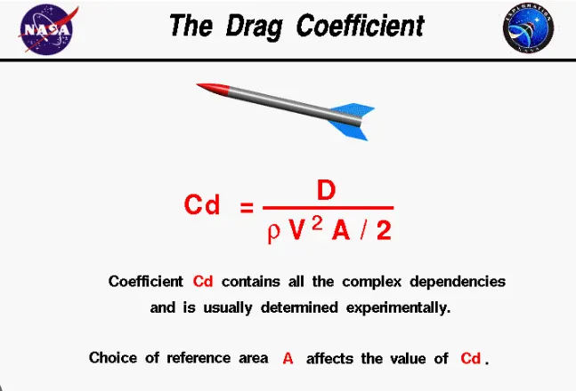
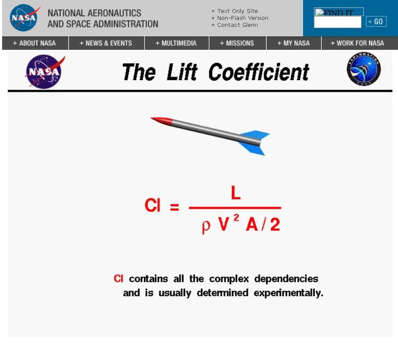
Cd and Cl Equations

PROCEDURE:

BASELINE MESH:

SOLVING AND MODELLING APPROACH:

1. V=25 m/s
2. Computational Domain:

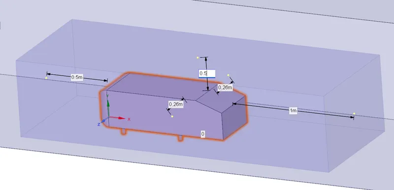
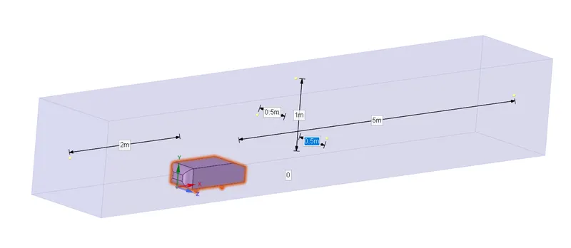
The body was split into half using split command.

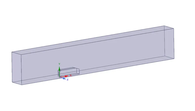
PREPROCESSING AND SOLVER SETTING:

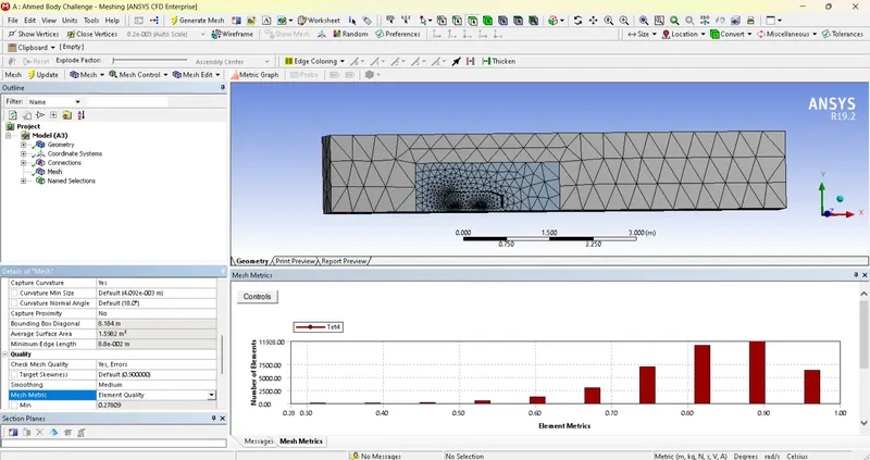
MESH SETTING:

1. Triangular-Tetrahedral Mesh pattern is selected.
2. Element size is set to default

SOLVER SETTING (Steady State):

1. Model: Density based – Steady state flow, Viscous -SST K-Omega selected.
2. Materials= Air
3. Boundary Conditions:
   1. Inlet- velocity with magnitude 25m/s and temperature to 300K.
   2. Outlet- Pressure based- Gauge pressure 0
   3. Cylinder wall- No slip condition and stationary boundary.
   4. Symetric wall- Symmetry Boundary Condition.

4. Reference values -
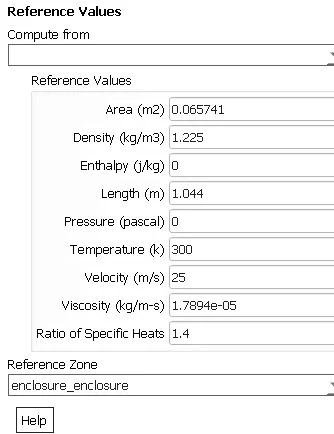
5. Method: SIMPLE Algorithm with default wall conditions.
6. Defined lift and drag coefficients across car wall.
7. Selected Hybrid Initialization and Initialized for 10 iterations.
8. Defined new contour plots for velocity and pressure and vector plot.
9. Set 500 iterations and run calculations.

REFINED MESH

SOLVING AND MODELLING APPROACH:

1. V=25 m/s
2. Computational Domain:

The body was split into half using split command.

PREPROCESSING AND SOLVER SETTING:

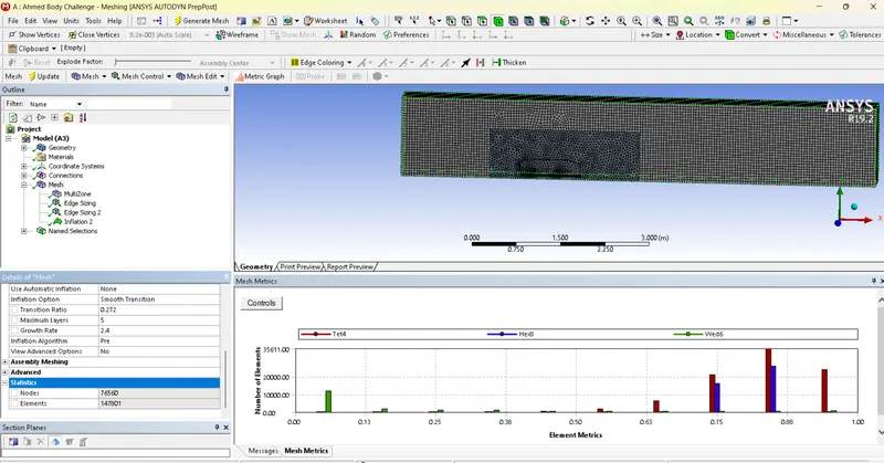
MESH SETTING:

1. Hex Mesh pattern is selected outside body.
2. Element size is set to 0.45m.
3. 10 inflation layers with base layer mesh height set to 0.0000144 m and growth rate of 1.5 is given around the cylinder.

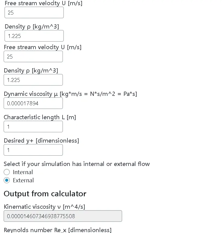
SOLVER SETTING (Steady State):

1. Model: Density based – Steady state flow, Viscous -SST K-Omega selected.
2. Materials= Air
3. Boundary Conditions:
   1. Inlet- velocity with magnitude 25m/s and temperature to 300K.
   2. Outlet- Pressure based- Gauge pressure 0
   3. Cylinder wall- No slip condition and stationary boundary.
   4. Symetric wall- Symmetry Boundary Condition.

4. Reference values -
5. Method: SIMPLE Algorithm with default wall conditions.
6. Defined lift and drag coefficients across car wall.
7. Selected Hybrid Initialization and Initialized for 10 iterations.
8. Defined new contour plots for velocity and pressure and vector plot.
9. Set 350 iterations and run calculations.

RESULT:

BASELINE MESH

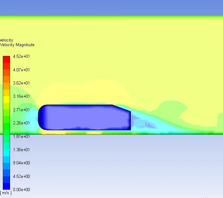
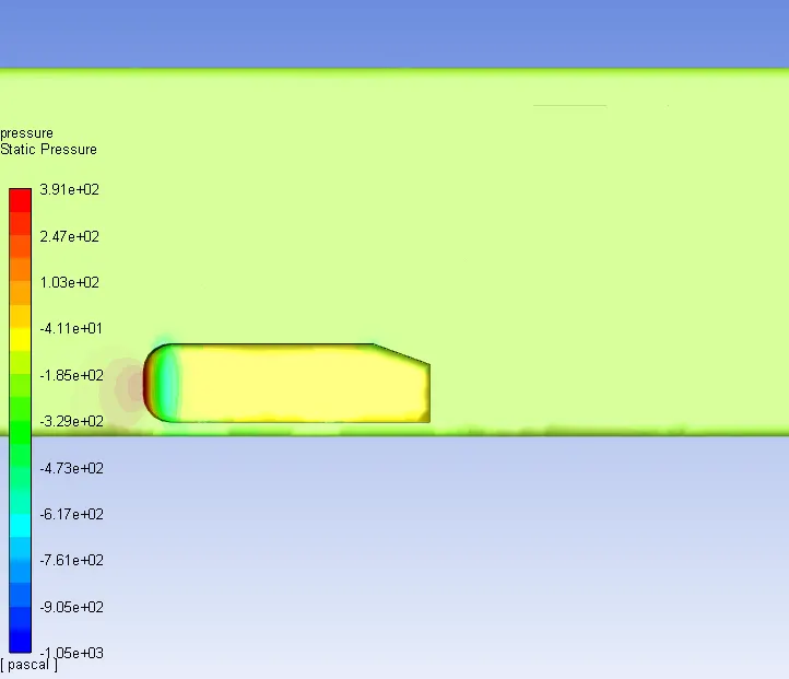
1. Steady state convergence, velocity, pressure contour plots and vector are made.
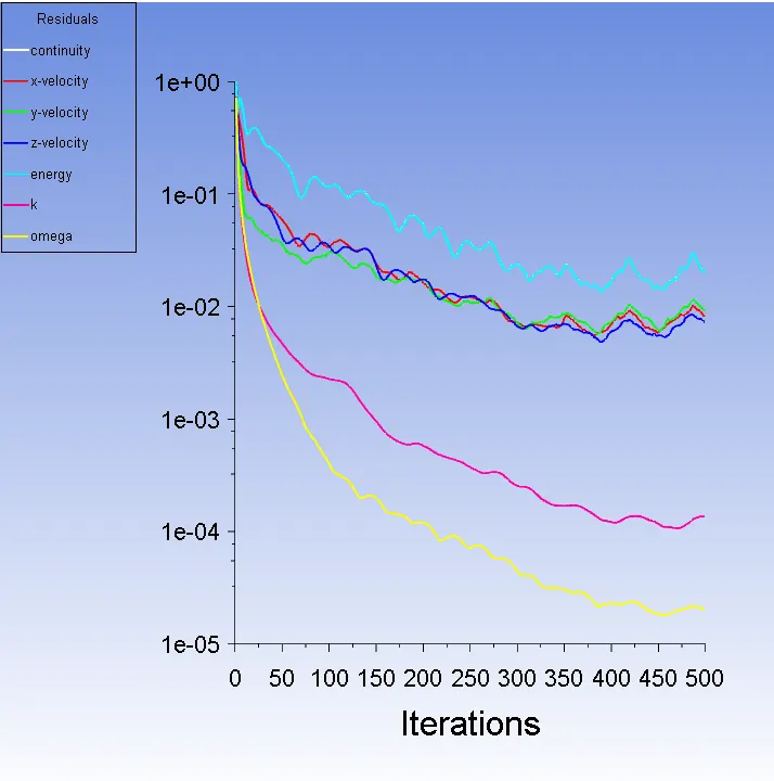
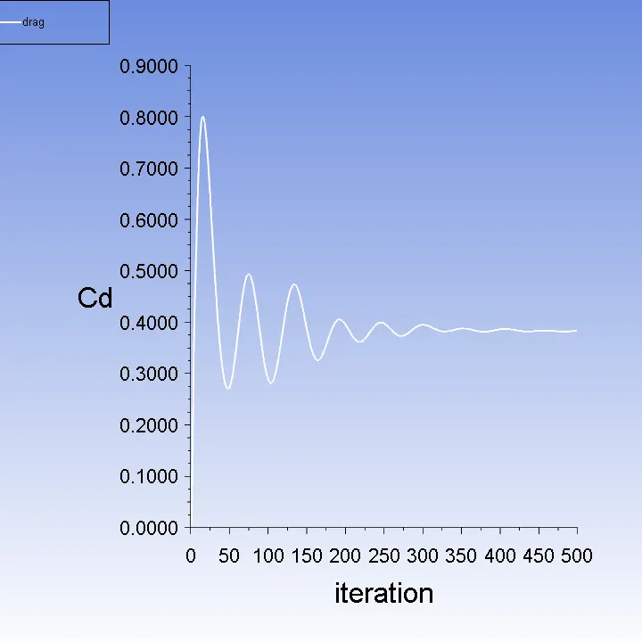
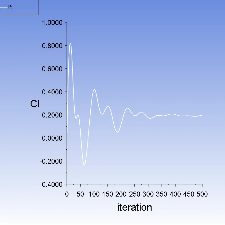
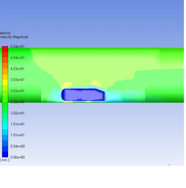
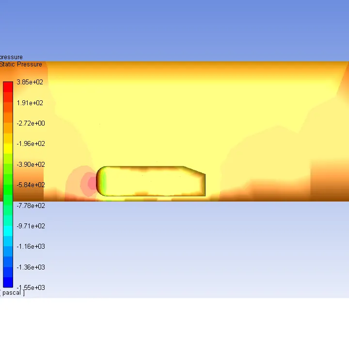
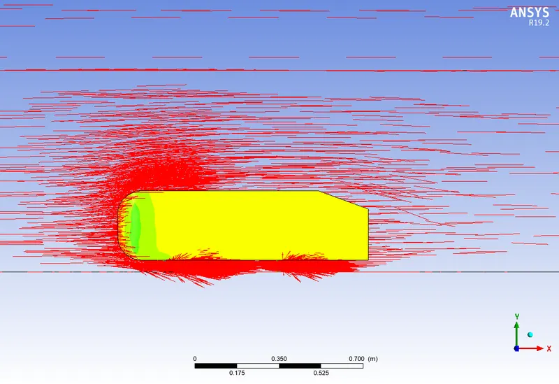
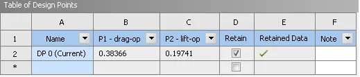
2. Value of Cd and Cl.

REFINED MESH

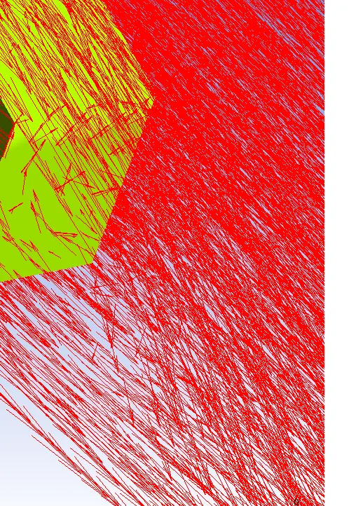
• Steady state convergence, velocity, pressure contour plots and vector are made.

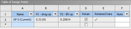
• Value of Cd and Cl.

CONCLUSION:

It is noted that from table that Using Grid dependency test Refined mesH with Y+ calculation yielded better results in Cd and Cl when compared to Baseline mesh.

It can be noted from the below mentioned table that Error percentage was reduced from 16.37% to 5.45% using mesh refinement.

Mesh Refinement	Cd	Cl	Cd Error %
Baseline Mesh (SST K-Omega)	0.384	0.197	16.37%
Refined Mesh (SST K-Omega)	0.312	0.208	5.45 %

IN NOTE OF WAKE FORMATION : It can be noted that in refined mesh the recirculation and vorticity of velocity vectors are captured in better way.

Note on boundary layer and flow separation and reason behind negative pressure in the wake region:

Boundary Layer: When a fluid flows over a plate, the velocity of the near most layer of the fluid is zero, relative to the plate. And the velocity of the subsequent layers keeps on increasing until the magnitude is equal to that of the free stream velocity. The boundary layer can be viewed as the thin layer of the fluid along the surface of the plate where the effect of viscosity is present, and the vorticity is also seen. The thickness of the boundary layer is said to be the distance between the plate and the layer of fluid until the velocity of the fluid layer has reached to about 99% of the free stream velocity. The following picture depicts the growth of a boundary layer on a flat plate

Flow Separation: Boundary layer separation is the detachment of the boundary layer from the surface into a region of recirculating flow immediately a body that is in relative motion with the fluid. When there is a large enough adverse pressure gradient, the boundary layer gets separated and the speed of the boundary layer relative to the surface will be stopped and will have reversed direction. The flow will be detached from the surface and it becomes eddies or vortices. This phenomenon would cause the negative pressure in the wake region and hence, the flow separation results in the reduced lift and an increased pressure drag

REFERENCES:

1. Anderson J.D,”Fundamentals of Aerodynamics”, 2^nd Ed,Ch.3:pp.229
2. Shames I.H,”Mechanics of fluid”, 3^rd, Ch.13:pp.669-675
3. http://foramehelp.blogspot.com/2014/03/drag-cofficient-definition-equation.html
4. https://volupe.se/en/wall-y-calculator-when-meshing-a-geometry-for-cfd-analysis-this-handy-volupe-calculator-computes-the-height-of-the-first-mesh-cell-off-the-wall-required-to-achieve-a-desired-y-using-flat-plate-boun/