Week 3 - External flow simulation over an Ahmed body.
Aim:
Simulation of External flow over the Ahmed body is conducted in this challenge. Parameters such as coefficient of lift and coefficient of drag are estimated and validated. The wake region is investigated. The Grid Independence test is conducted.
Ahmed's body and its importance:
The Ahmed body is a geometric entity that represents a standard passenger car. The geometry was first proposed by Ahmed and Ramm in 1984 and was extensively used to study the effects of the geometry on the wake region. Over the years, numerous studies have been conducted on the Ahmed body computationally and experimentally using wind tunnels. Since a lot of data is available on the Ahmed body, today the geometry is primarily a validation tool for CFD codes. The geometry of Ahmed's body is shown below:
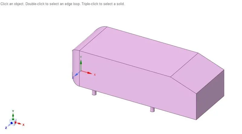
Variation of the slant angle (ψ) at the back of the geometry is the primary parameter in the characterization of the wake region. It has been found that ψ = 30 deg is the critical value of the slant angle. A pair of counter-rotating vortices is generated for Ahmed bodies, whose ψ is below 30 deg. These vortices help in preventing the separation of flow along the slant surface. Above a ψ of 30, separation of flow occurs somewhere along the slant, and flow develops into a relatively larger recirculating region in the wake.
Importance of Ahmed's body
The drag force is an important factor considering fuel consumption. As the drag force increases the fuel consumption also increases which in turn becomes expensive for the car owners. As the burning of fossil fuels becomes an issue, manufacturers are pressing for fuel-efficient cars. One of the main factors considering whether the car is fuel-efficient or not is the car's geometry.
Complex-shaped cars are very challenging to model and its difficult to quantify the aerodynamic drag computationally. The Ahmed body is a benchmark model widely used in the automotive industry for validating simulation tools.
Negative pressure in the wake region:
The moment the flow hits the front the pressure gets increased, then according to Bernoulli’s theorem that flow gets divided between the upstream and downstream of Ahmed's body having high and low velocity respectively.
As the flow gets unable to navigate the surface, the upper layer i.e free velocity goes straight. The boundary layer experience a disruption making some of the particles get goes straight some get separated and take the reverse direction, and only a few particles cope with the contour of the body. this creates a low-pressure region that has negative pressure at the back.
On the other hand at the base side, the pressure is high compared to the overhead side of Ahmed's body but the pressure keeps on increasing as it can seem to from the contour. The already created low-pressure region by the upstream flow causes the flow to move straight.
The pressure region also causes some air molecules to get reattached to the Ahmed body which makes a recirculation region. The low-pressure region at the rear cause a pressure drag. As the flow from the front gets heavily attracted gets attracted toward low pressure.
When the air moving over the vehicle is separated at the rear end, it leaves a large low-pressure turbulent region behind the vehicle which is known as the wake. This contributes to the formation of pressure drag which affects the vehicle's performance.
When the vehicle is moving at a certain velocity the fluid imparts viscous force to the vehicle as long as it is in the viscous sublayer of the boundary. When the fluid reaches the rear end of the vehicle it gets detached from the surface of the body causing negative pressure in the wake region. The movement of the fluid around the vehicles depends on the geometry of the car and the Reynolds number.
Significance of point of separation:
The point of separation will occur when there is a discontinuity in the surface or a region of the negative pressure gradient (a sharp end or rear portion of the car).
When the flow is attached to the body of the vehicle the viscous force will increase which will increase the pressure and decrease in velocity before the rear end of the vehicle. As soon as the air encounters the sharp turn causing the velocity decreases resulting in the negative pressure region which is in the wake region. The recirculation region happens beyond the point of separation.
If the rate of change of pressure is large the mixing process will not occur and the boundary layer flow stops.
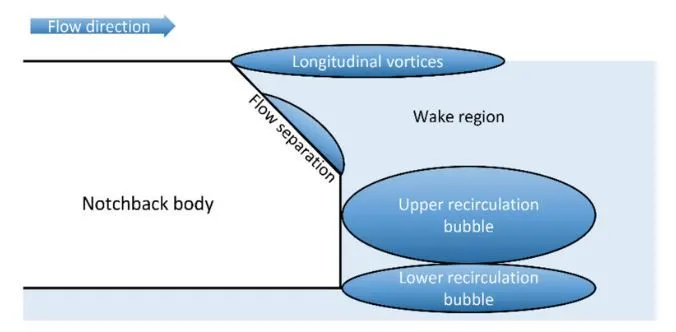
A flow separates as soon as it detaches from a surface into a wake. It occurs when the flow slows and there is an increase in the pressure after passing a bluff or streamlined body.
The position at which the boundary layer leaves the surface of a solid body. It may occur with the laminar flow (laminar separation) or when the boundary layer is turbulent (turbulent separation). Separation is sometimes followed by a reattachment of the flow.
Flow separation or boundary layer separation is the detachment of a boundary layer from a surface into a wake. Separation occurs in flow that is slowing down, with pressure increasing, after passing the thickest part of a streamlined body or passing through a widening passage. For example, Flowing against an increasing pressure is known as flowing in an adverse pressure gradient.
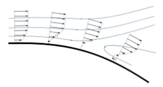
The above figure shows that at the point of turning the flow gets separated from the boundary layer and there is a region of recirculation after which the flow attaches itself to the boundary layer.
To reduce the separation of fluid from the boundary layer, it is advisable to have a smooth edge to reduce the effect of drag on the vehicle.
Case setup in Ansys Fluent:
In this challenge, the study is performed on Ahmed's body whose slant angle is 20 degrees using Ansys fluent. The freestream speed of flow is taken as 25 m/s and the fluid is 'air'. The wake region is analyzed with contours and vector plots of velocity at certain probe locations behind the geometry. Parameters such as coefficient of lift, coefficient of drag, and point of separation of flow are estimated.
Since the Ahmed body is symmetric about the X-Y plane (shown above), the body is to be split into two symmetric halves and the 'symmetry' boundary condition is to be applied. This helps to save a lot of computational cells that can be used to further refine the wake region.
The given problem is external aerodynamic simulation. A wind tunnel is created over Ahmed's body using the 'Enclosure' option in Spaceclaim. This outer enclosure contains a smaller, inner enclosure (for local refinement) which in turn contains the surface of the Ahmed body. While creating the enclosures, the 'Interference' option was used to remove any geometric interference and common regions created by the double enclosures. The 'topology' option is set to 'Share' to ensure data is shared between different enclosures.
External flow simulation over Ahmed's body by creating a two-closure.
Outer Enclosure:
The outer enclosure is of bigger dimensions to make the inflow and outflow boundary conditions not be influenced by the presence of the Ahmed body. But it is impractical to make the whole domain thoroughly refined because it would result in a waste of computational resources. Hence a smaller inner enclosure is created for the purpose of local refinement. It is of immense importance to refine the mesh much more, closer to the geometry which is shown below.
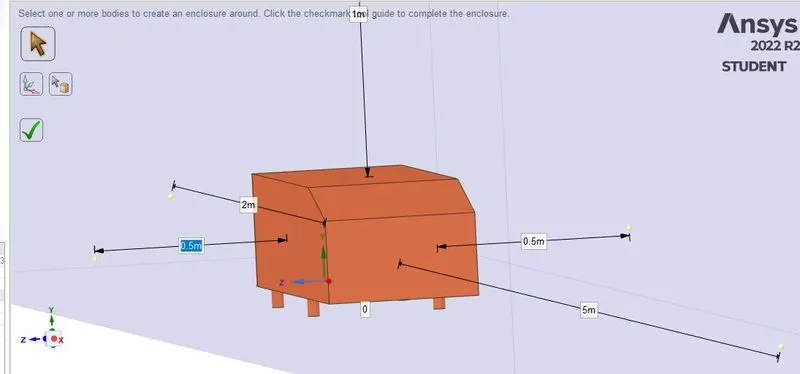
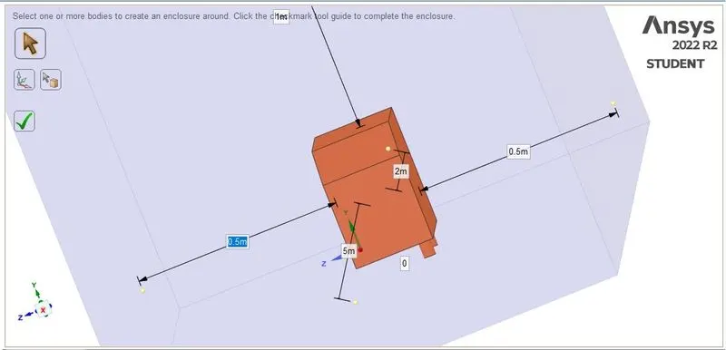
A wind tunnel has to be created around Ahmed's body, there are multiple methods to achieve this, but the easiest is using the enclosure tool in ANSYS to generate the tunnel. The inlet of the wind tunnel is 2 meters from the front of the Ahmed body, the outlet is 5 meters from the back of the body. The height of the enclosure is 1 meter above Ahmed's body while the width is 0.5 m from the side of the body and the bottom is zero. The enclosure is checked for Interference and it is repaired as well.
Inner Enclosure:
Further enclosures have been created for mesh refinement. The inlet of the wind tunnel is 0.5 meters from the front of the Ahmed body, the outlet is 1 meter from the back of the body. The height of the enclosure is 0.5 meters above Ahmed's body while the width is 0.25 m from the side of the body and the bottom is zero.
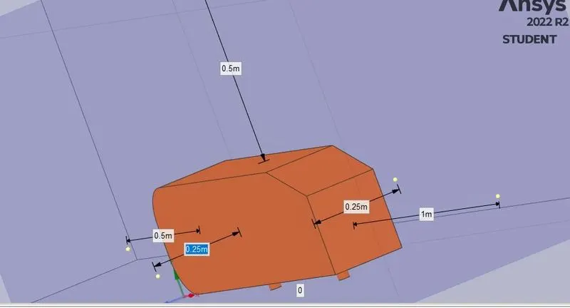
Since this is a complex simulation and the Ahmed body is symmetrical along the x-axis, the geometry was split into two along the x-axis using ANSYS's split tool.
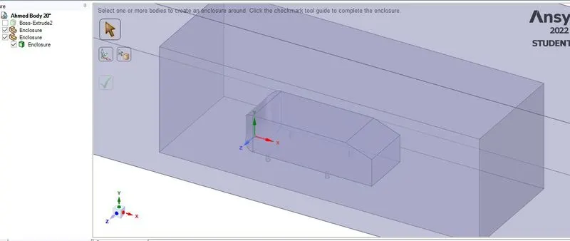
This is the geometry after the splitting:
Meshing:
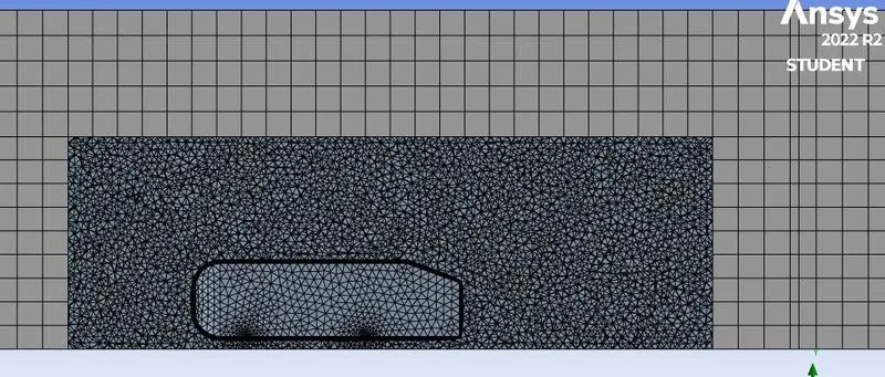
Next, the mesh module is opened. Since the geometry of the outer enclosure is made of straight lines, the 'hex' mesh is used. The inner enclosure holds the surface of Ahmed's body and hence is 'triangle dominant'. The 'Multizone' mesh method is applied to the outer enclosure to connect different mesh types. The base mesh size is set to 0.1 meters.
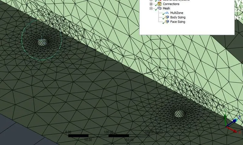
The inner enclosure is given 'mesh body sizing' and is set to a size of 0.05 meters. Mesh 'face sizing' with a size of 0.005 meters is given on the cylindrical stands of the Ahmed body to prevent geometry distortion at the stands. To capture the near-wall physics accurately, a boundary layer mesh (Body fitted Mesh) (or) Mesh inflation is provided to the geometry. To come up with the right mesh size, the following calculations are done. Shown below is the mesh obtained.
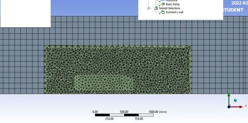
Sizing: It is defined as increasing the number of elements by decreasing the element size. The element size of the second Enclosure is 0.05 m
Element size for the first enclosure: 100 mm
Element size for the second enclosure: 50 mm
Element size of pillars of Ahmed's body: 5 mm
Number of elements : 1,68,083
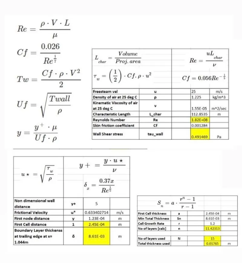
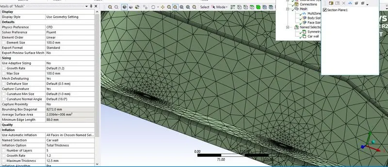
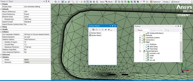
To capture the near-wall effects, the `k-omega` SST Turbulence model (y+ range 1 to 5) is preferred. The mesh inflation option is set to 'Total thickness. Two parameters are required: The total thickness of inflation and the number of inflation layers. Firstly, the boundary layer thickness at the end of the Ahmed body is calculated using the boundary layer formula for turbulent flow over a flat plate. Considering the y+ for the problem as 5, the first layer thickness is calculated. Now, the number of inflation layers can be calculated using the Sum of n terms of the GP formula.
Y+ Concept:
The behavior of the flow near the wall is a complicated phenomenon and to distinguish the different regions near the wall the concept of wall Y+ has been formulated. Thus Y+ is a dimensionless quantity and the distance from the wall is measured in terms of viscous lengths.
Fluent:
Next, Fluent is opened and a meshed check is performed. A pressure-based steady-solver is used for the case as the flow speed of 25 m/s is well below Mach 0.3. At the reference values, the projected area, length, velocity, and region from which flow occurs are specified. The turbulence model is set to k−omega SST. Material is 'air'. The boundary conditions are specified next.
Boundaries:
inlet - velocity inlet
outlet - pressure outlet
wall-car - wall (no-slip)
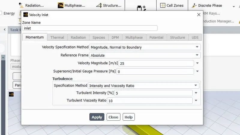
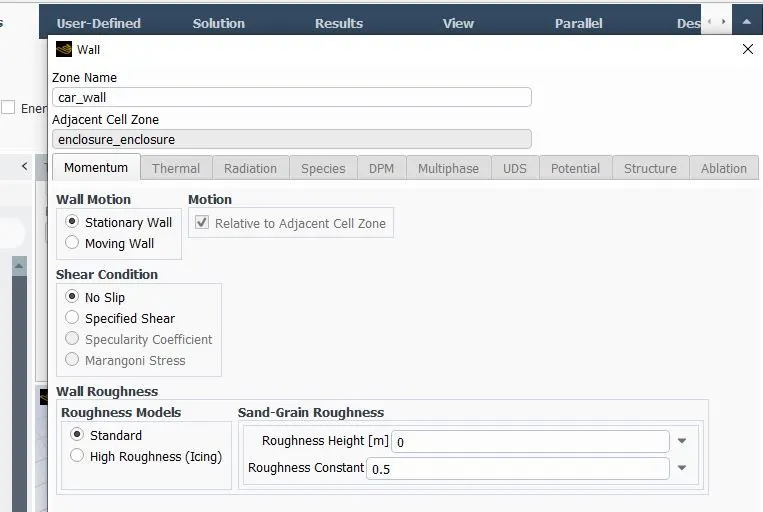
Materials
The existing material's (air) properties were used and were left unchanged.
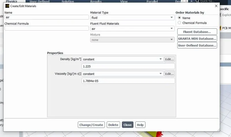
We know, Reynold's Number
Re = ρ⋅u⋅D/μ
where, ρ is density (kg/m^3), u is inlet freestream velocity (m/s), D is the characteristic length of the Ahmed body (m) and μ is the kinematic viscosity kg/(m.s)
Viscous
k-omega SST was used for all simulations for this project due to its excellence in solving external flows and wake regions.
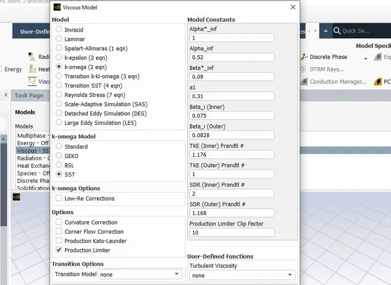
Hybrid initialization is selected and the solution is initialized by hitting t=0
The problem is then initialized using the Hybrid solver. Create a surface plane to see the contours. Plots such as coefficient of lift, coefficient of drag, pressure contours, velocity contours, and vector plots are set up before the simulation. Finally, the case is run for 500 iterations.
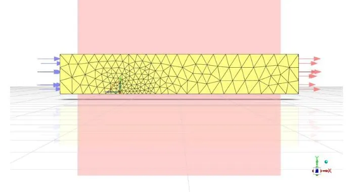
Creating a cut plane to see the velocity change along Ahmed's body:
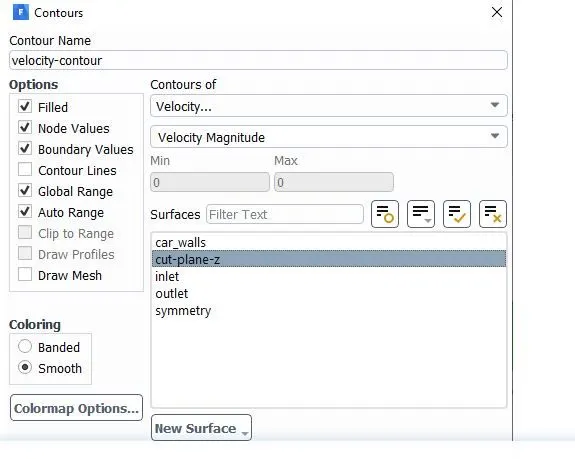
Creating a contour plot:
Convergence:
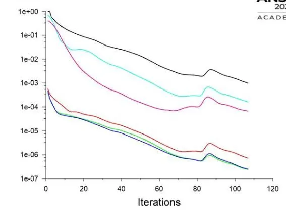
The number of iterations was set to 500.
But it is observed that the residuals have fallen below the specified tolerances and the solution attains convergence in ~110 iterations.
Reports:
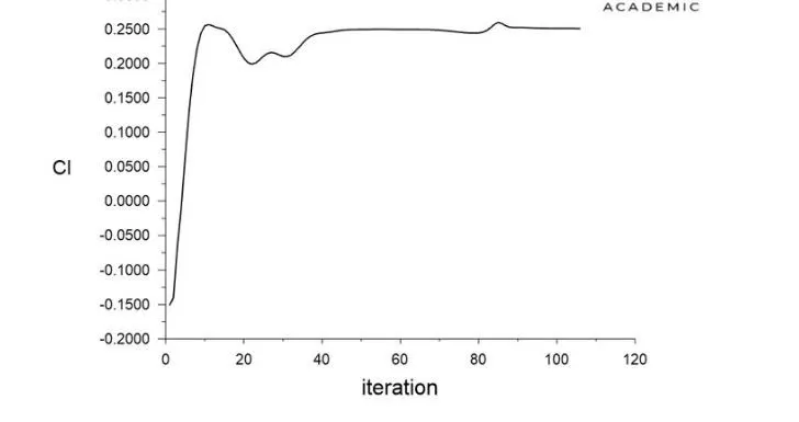
1. Lift Coefficient of wall-car
2. Drag Coefficient of wall-car
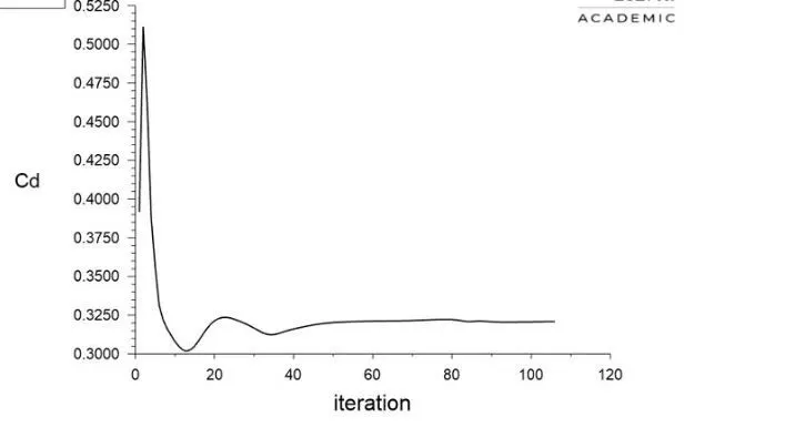
The formation of the low-pressure wake region dictates how high is the drag coefficient. The steady-state drag coefficient is found to be 0.3296. This result can be validated from (0.33) with an error of 3.04%.
The formation of vortices in the wake results in the lift. The steady-state lift coefficient is found to be 0.2504.
The flow separation occurs right at the end of the slant surface at the rear of the geometry. This flow separation results in a recirculation region of low pressure and determines the coefficient of drag of the body.
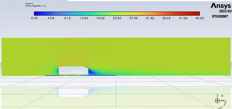
3. Velocity contours:
Zooming in,
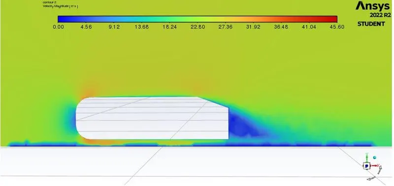
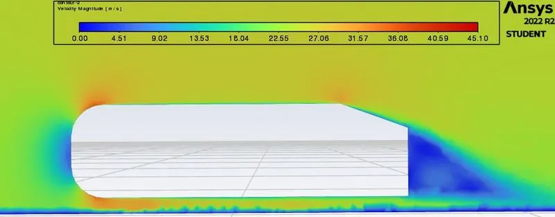
The contours are generated on an X-Y plane at Z = 0.
Just behind the slanted surface of Ahmed's body, a recirculation region is formed. This will be demonstrated more clearly by the vector plots in the coming section. The recirculation region has a lower-pressure core and is represented by the light green patches in the contour. The scale defined in the contour represents the gauge pressure and hence shows negative pressure values at the recirculation region.
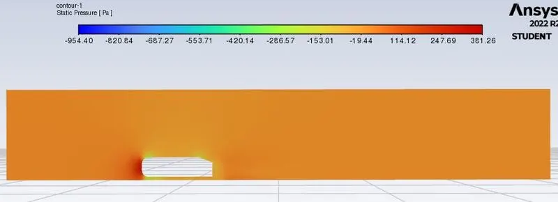
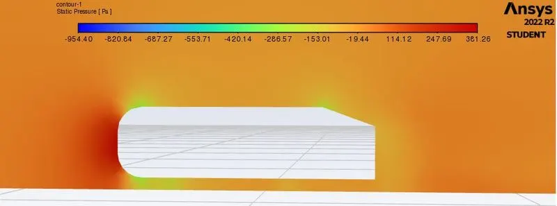
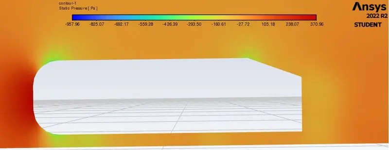
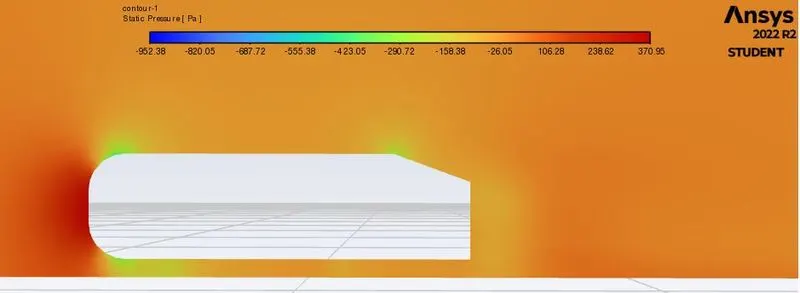
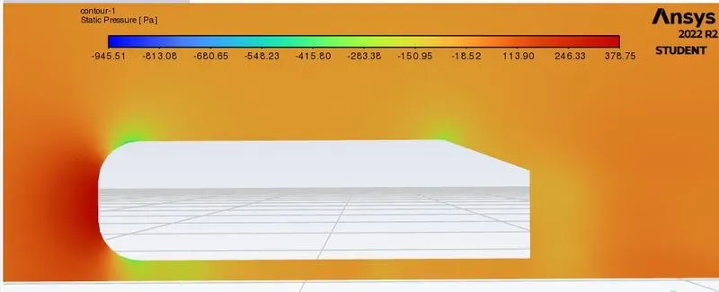
The pressure is maximum at the leading boundary of the Ahmed body because the flow is stagnated here. Also, at points where there exists curvature such as the filleted region at the leading boundary and the sharp beginning of the slant, there exist local low-pressure regions due to a sudden change in the geometry.
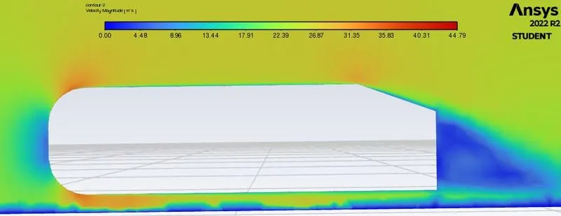
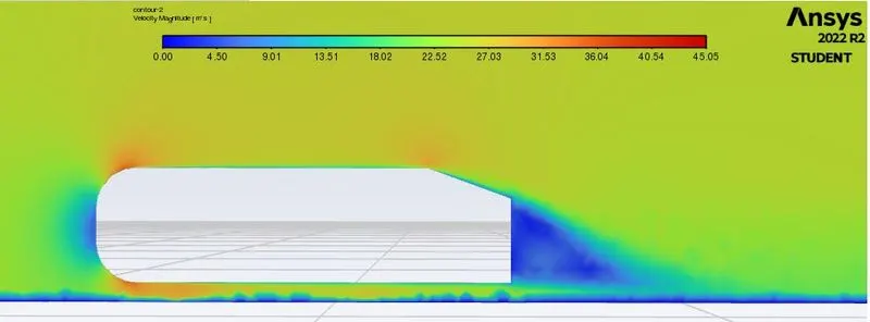
The velocity contour shows the flow over the slanted region. The flow does separate till the end of the slanted surface, after which separation occurs. A low-velocity region is formed at the recirculation region. This low-pressure region extends far into the wake of the car along with the formation of counter-rotating vortices which is shown in the next section.
At the different curvatures on the surface of the Ahmed body, where local low pressure exists, the regions have relatively higher velocities.
Zooming in further,
Wake region:
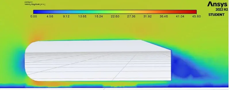
The wake is clearly visible.
4. Vector plot:
These were taken in CFD - Post. The background contour is the velocity contour.
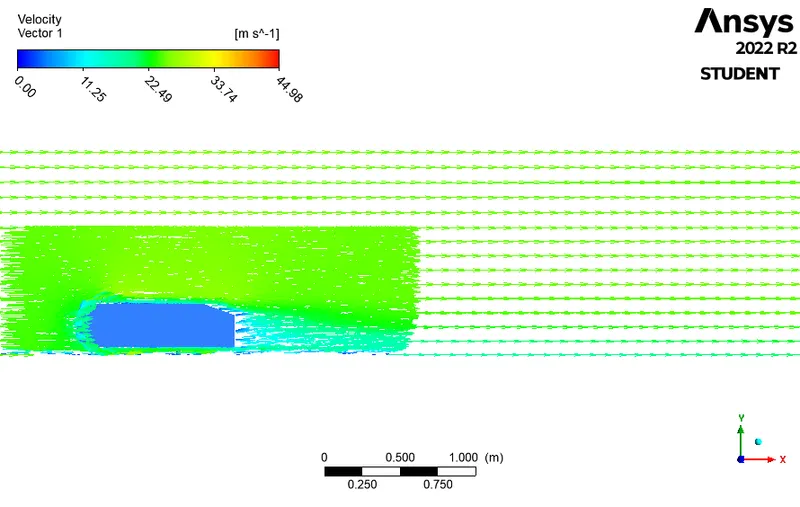
Zooming in,
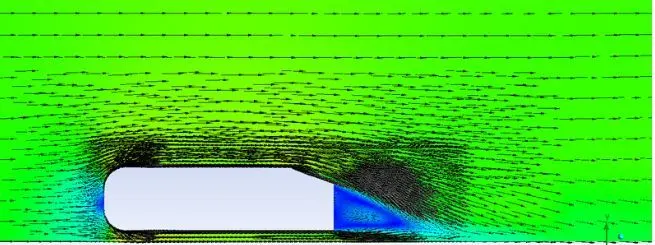
Zooming in further near the wake region,
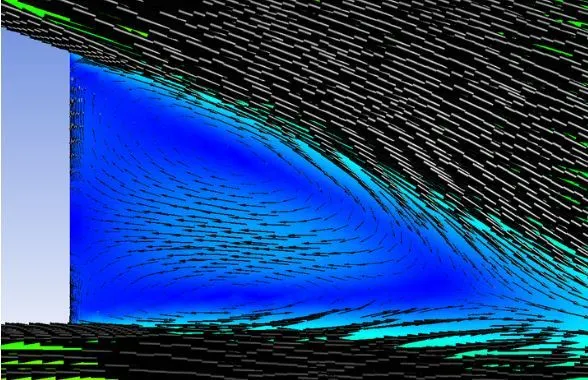
Switching the type of arrow to see the lines more clearly,
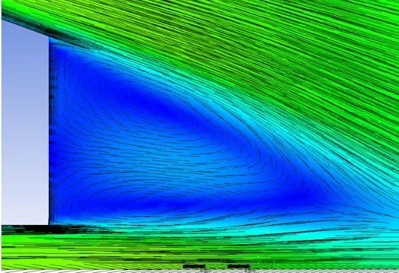
Two distinct regions can be spotted behind the Ahmed body with two vortices (seen from this view) or recirculating regions behind the Ahmed body.
The vector plot shows the direction of flow at all locations. It is colored by velocity. The recirculation region is clearly seen in the images shown above.
This recirculation region further develops into a pair of counter-rotating trailing vortices that have a low-pressure region in the core. These vortices are visualized better in the next section.
5. Vector plots at Y-Z Plane probes:
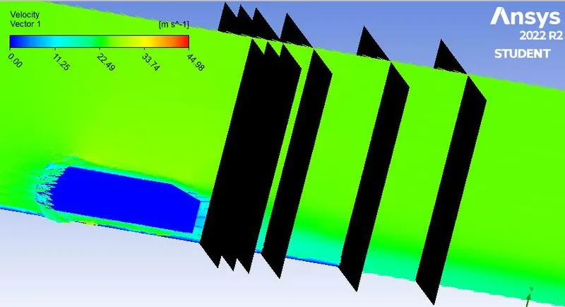
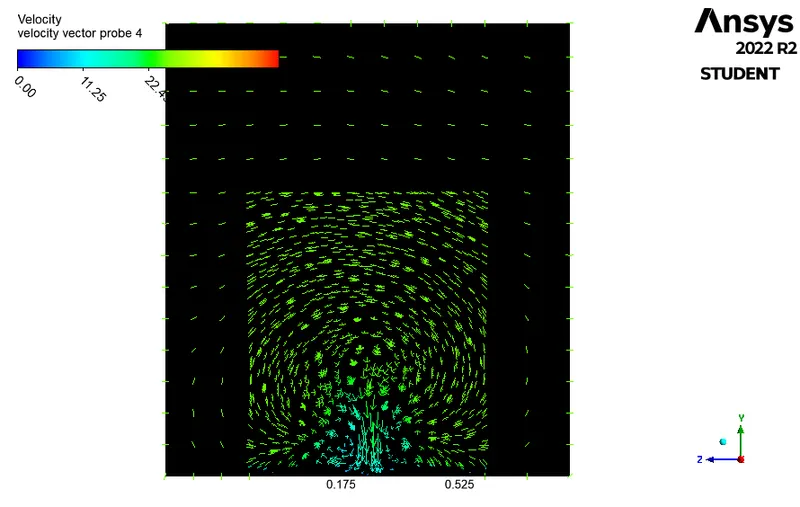
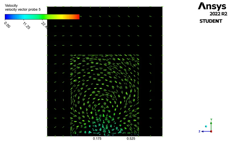
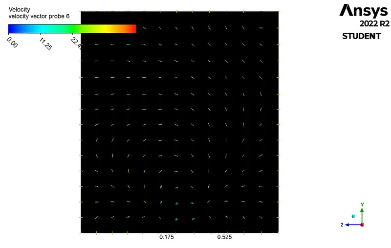
These vector plots are generated at specific Y-Z plane probes as shown below at distances 1.1 m, 1.2 m, 1.3 m, 1.5 m, 2 m, and 2.5 m respectively from the origin. The Origin is located at the front end of Ahmed's body.
Probe 1:
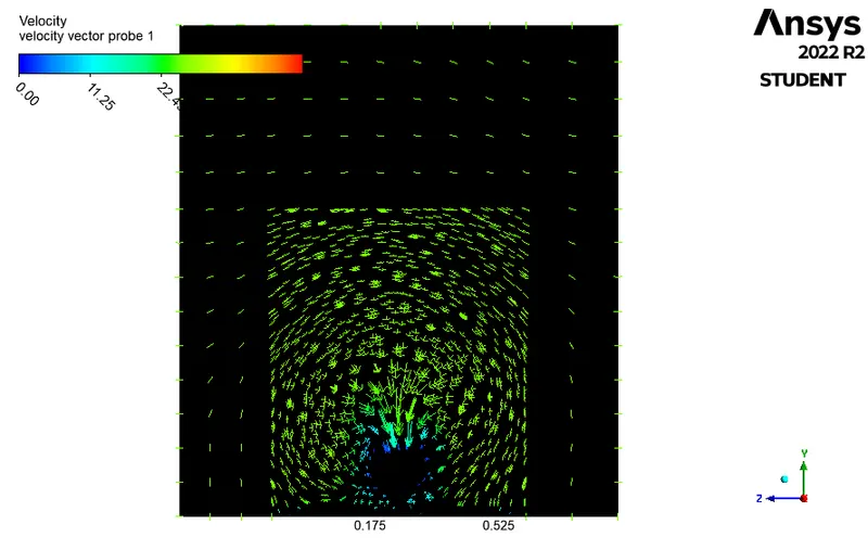
Probe 2:
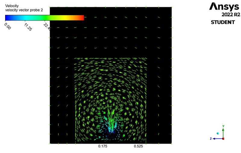
Probe 3:
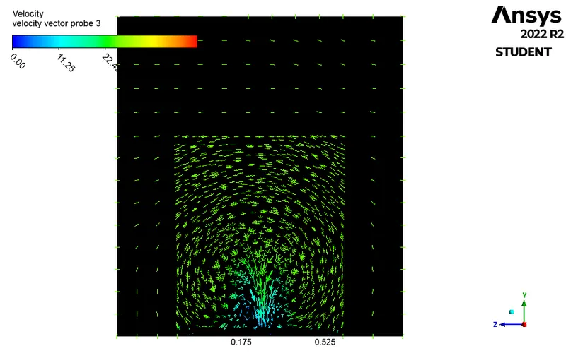
Probe 4:
Probe 5:
Probe 6:
It is observed that with increasing distance in the wake, the vortices become fully developed. The distance up to which the vortices influence the wake is slightly above 2 meters.
It is to be noted that the images shown above represent only one vortex as the geometry was split and symmetry BC was applied. Hence, it can be assumed that a similar vortex is formed on the right-hand side of the displayed vortex.
Eventually, the wake dies out and the flow is reattached. At a distance of 2.5 meters, it is observed that the flow is the usual freestream flow.
6. Velocity Profile at various Line probes:
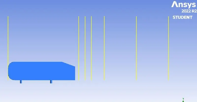
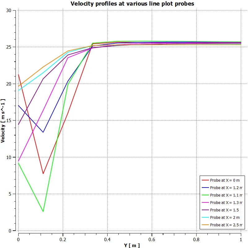
Various line probes are drawn at distances of 1.1 m, 1.2 m, 1.3 m, 0 m, 1.5 m, 2 m, and 2.5 m respectively from the origin. The Origin is located at the front end of Ahmed's body.
The velocity profile drawn at each of these lines probes wrt the distance in the Y direction.
For these three probes (1.1 m, 1.2 m, 1.3 m), the velocity reduces from the freestream speed to a minimum at the recirculation region and climbs steadily up to a value after which the influence of the wake is not present. From here, the gradient in the velocity is very small and it attains the free stream speed. For the probe at X=0, the flow reduces from freestream to 0 at the stagnation point and then follows the same trend as before.
The rest of the probes that are present in the influence of the wake, have velocities lesser than the freestream speed and gradually rise to the freestream speed. No points of minimum speed are observed at these probes.
Pressure contours:
Zooming in,
Zooming in further,
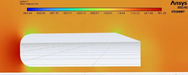
There is a high-pressure region at the front of the body due to how flowing air is accumulated at the front.
The pressure is negative in some regions, this is not an error in the simulation but rather how ANSYS and Fluent function. The "pressure" displayed in ANSYS is actually gauge pressure, the gauge pressure is 0 when the total pressure is the atmospheric pressure. In this case, the "pressure" being negative is merely the pressure dropping below atmospheric in some regions.
Grid Dependence Test
A Grid Dependence Test is used to ascertain whether the final values of the solution are dependent on the mesh or not. This is an important test to ensure the simulation results are correct.
The test will involve 3 different simulations - where the mesh becomes finer. To capture the near-wall effects, the `k-omega` SST Turbulence model (y+ range 1 to 5) is preferred. The mesh inflation option is set to 'Total thickness. Two parameters are required: The total thickness of inflation and the number of inflation layers are considered the same for all 4 cases.
The modeling approach is the same as the previous case (Baseline simulation)
Ahmed's body is loaded into the Spaceclaim. Two enclosure is drawn across Ahmed's body. Now the geometry is loaded for meshing. Named selection is created for the enclosure viz; inlet, outlet, symmetry. To create the named selection for the car the enclosure faces are hidden and the box select is selected from the meshing toolbar and the (car wall) name is given to it. Ansys Fluent window is opened and the geometry is loaded. Steady-state, the density-based solver is selected. Reference values are updated as per the prescribed conditions. In the inlet boundary condition, the inlet velocity is 25 m/s. Drag-coefficient plot and the lift-coefficient plot is created by setting the reference as (car walls). Hybrid initialization is selected. The solution is initialized by hitting t=0. The cut-plane-z is created along Ahmed's body. The velocity contour and pressure contour are created along the cut-plane-z. The animation video is created for the velocity contour.
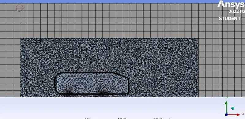
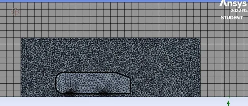
The first simulation runs successfully. The geometry is loaded into SpaceClaim. The region of local refinement is created along Ahmed's body. As the body is perfectly symmetric, the simulation is executed by considering only half the body. This is the best practice where we can save on the number of cells and get the results faster as well. The geometry is loaded for meshing. The multizone method is selected for the outer enclosure to provide hexahedral mesh which provides accurate results in simulation. The element size for the different outer enclosures will vary from (100mm and 90mm), the element size for the different inner enclosures will vary from (50mm, 40mm, and 25mm), and the element size of the leg of Ahmed's body will be 5mm, the first layer thickness, inflation layer, and the maximum thickness will be same. The rest procedure is the same as above, the necessary contour plot and graphs have been uploaded respectively.
| CASES | Outer Enclosure mesh size (mm) | Inner Enclosure mesh size (mm) | Face Sizing mesh size (mm) | Number of Elements | Turbulence Model |
| Baseline | 100 | 50 | 5 | 168083 | K-omega SST |
| Grid 1 | 100 | 40 | 5 | 266999 | K-omega SST |
| Grid 2 | 100 | 35 | 5 | 362447 | K-omega SST |
| Grid 3 | 100 | 31 | 5 | 489426 | K-omega SST |
NOTE: Further refinement cannot be done because the cell count exceeds 500000 cells which cannot be solved in the academic version.
Case Grid 1:
Mesh
Pressure Contour
Velocity Contour
Case Grid 2:
Mesh
Pressure Contour
Velocity Contour
Case Grid 3:
Mesh
Pressure Contour
Velocity Contour
The case is set up using meshes of increasing local refinement in an attempt to get mesh-independent results. The following are the results obtained for the combination of different mesh sizes. The maximum number of cells that can be used in the academic version of fluent is 512000 cells.
Grid 3 holds the maximum refinement and the cell count is close to the maximum value. The error in the drag coefficient obtained using grid 2 with the reference value(0.33) is 3.76%. Grid 1 produces an error of 3.33%. Hence, grid 1 and grid 2, both produce close values and both these results can be considered grid-independent.
| CASES | Coefficient of lift | Coefficient of drag | Error in the drag coefficient (%) |
| Baseline | 0.2463 | 0.36076 | 9.32 |
| Grid 1 | 0.2598 | 0.34096 | 3.33 |
| Grid 2 | 0.2504 | 0.32096 | 3.04 |
| Grid 3 | 0.2601 | 0.31024 | 5.98 |
Conclusion:
It can be inferred that the grid independence test is performed to know the smaller cell size for convergence.
Apart from mesh refinement, convergence depends on the Y+ value, and inflation layer, it is advisable to use k-ω-SST as the turbulence value because it calculates the values well near the wall.
As the setup is refined drag coefficient, and lift coefficient decrease.
Y+ plays an important role in determining the value of drag.
The negative pressure in the wake region is primarily because there is no flow in that region. This can be further attributed to various factors such as separation and recirculation which is evident from the vector plot near the wake region.
The point of separation occurs at the rear end of the vehicle, the separation occurs beyond this point where it can be observed that the flow recirculates and attaches it to the boundary layer.
The flow over the Ahmed body is conducted and the wake region is visualized using Vector and Contour plots and analyzed. The coefficient of drag and coefficient of lift is estimated. The point of separation and its influence is talked upon.
A grid Dependence Test was conducted and the test was successful, an additional observation was also made - the drag coefficient decreases as the number of elements increases. This decrease is very small and may be considered insignificant.