Week 3 - External flow simulation over an Ahmed body.

Aim: Performing a Grid dependency test on an Ahmed body and compare the results.

Introduction

The aim of this project is to simulate the Ahmed body for the Grid dependency, hence to see the effect of mesh sizing on the result of velocity and pressure distribution around the Ahmed Body.

Ahmed Body: It is a Generic Car body or simplified automobile body, which is being used in Automotive industries to simulate the flow characteristics around the Automobile. The fluid flow around the Ahmed body very accurately resembles the critical flow characteristics around the Automobile.

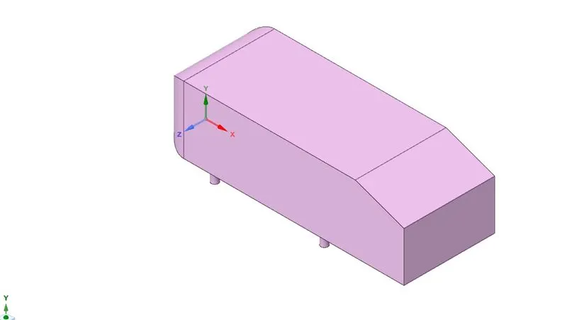
S.R. Ahmed developed the Ahmed specimen in his work “Some Salient Features of the Time-Averaged Ground Vehicle Wake” in 1984.

The simple geometrical shape has a Length of 1.044 m , Height of 0.288 m , and a width of 0.389 m . It also has 0.5 m cylindrical legs attached to the bottom of the body and the rear surface has a slant that falls off at 40 degrees.

IMPORTANCE OF AHMED'S BODY :

1. The three-dimensional flow around a vehicle has become a subject of significant importance in the automotive industry . One apparent technique of improving the fuel efficiency of a vehicle is to reduce aerodynamic drag force by optimizing the body shape .

2. Execution of fine aerodynamic design under stylistic constraints requires an immense understanding of the flow pattern phenomena and how the aerodynamics are impacted by changes in body shape.

3. The flow area which is presents the major contribution to a cars drag is the wake flow backing the vehicle . The point at which the flow seperates directs the size of the separation zone , and as a result the drag force . Clearly,a more accurate simulation of the wake flow.

4. Most cars have an average drag coefficient between 0.30 and 0.35 . Boxy cars have a higher number , like the HUMMER H2 vehicle at 0.57 , while more streamlined and agile cars have a lower number , like the Mercedes-Benz vehicle at 0.24 . Again , this is just an average measurement . The exact drag coefficient of a car varies with the Reynolds number and various other factors.

`Y^+` Concept:

The behaviour of the flow near the wall is a complicated phenomenon and to distinguish the different regions near the wall the concept of wall Y⁺ has been formulated. Thus Y⁺ is a dimensionless quantity, and is distance from the wall measured in terms of viscous lengths.

Where ,

ρ , µ are fluid density and viscosity ;

U is the free stream velocity ;

L is characteristic length ;

U_τ is frictional velocity ;

τ_ω is wall stress , C_f is skin friction coefficient

In this case , we take Y⁺=3 ;

From the calculation ,

We got first layer thickness is found to be 0.04 mm

PROCEDURE :

Solving & Modelling approach

STEP 1: Geometry creation

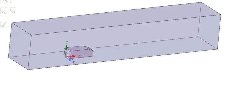
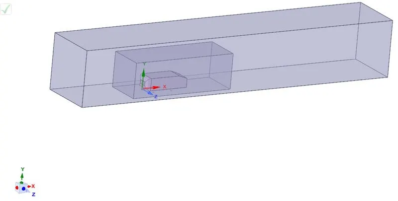
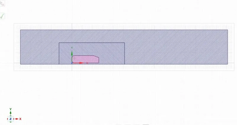
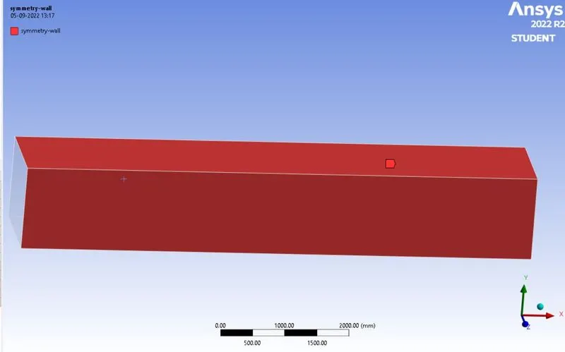
The Geometric model of Ahmed body and Geometry with all the dimensions are as shown in figures below. For Modelling Air-flow Over an Ahmed Body, it needs to be captured in enclosed control volume also known as the Computational domain. Figures below show the Enclosed computational domain for Ahmed body as well as Boundary conditions applied for the flow simulation. To save computational time and space, here the symmetric boundary condition is used as the model is symmetric. Below figure shows the sliced model which will be used further for meshing and simulation.

Geometry with outer enclosure:

Geometry with outer and inner enclosure:

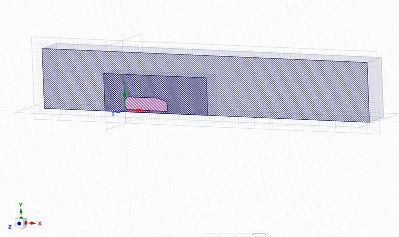
Sectional view using interference and share topology:

STEP 2 : MESHING

For this analysis , a baseline mesh along with 2 refinements has been done with the following features.

BASELINE mesh of the Computational Domain :

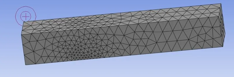
Section plane:

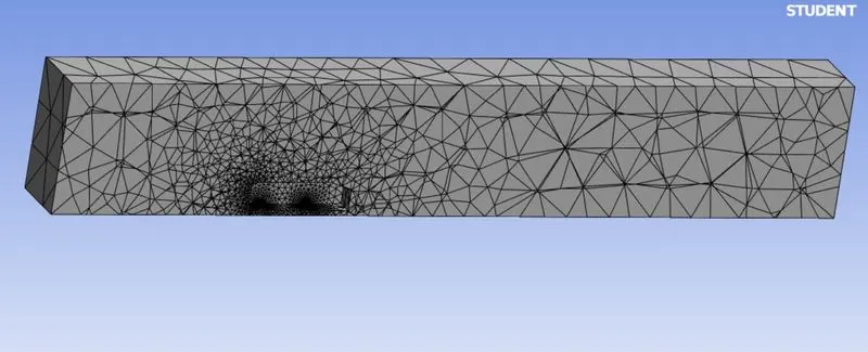
Refined mesh:

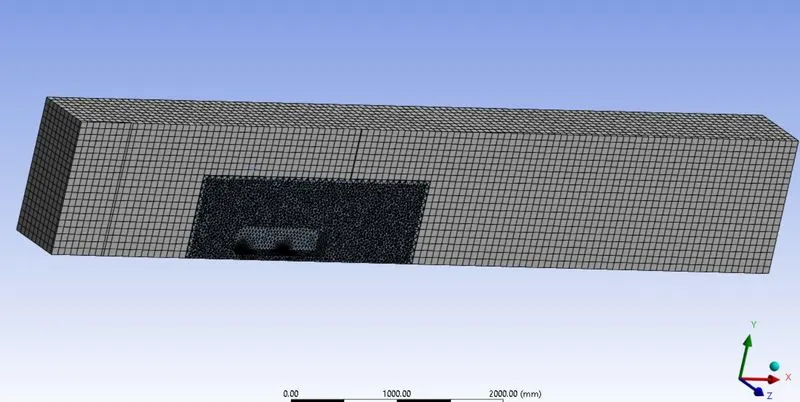
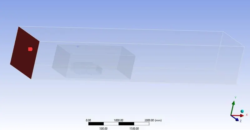
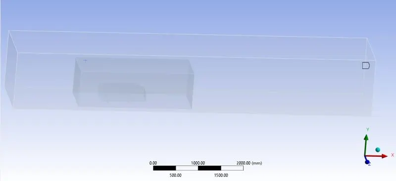
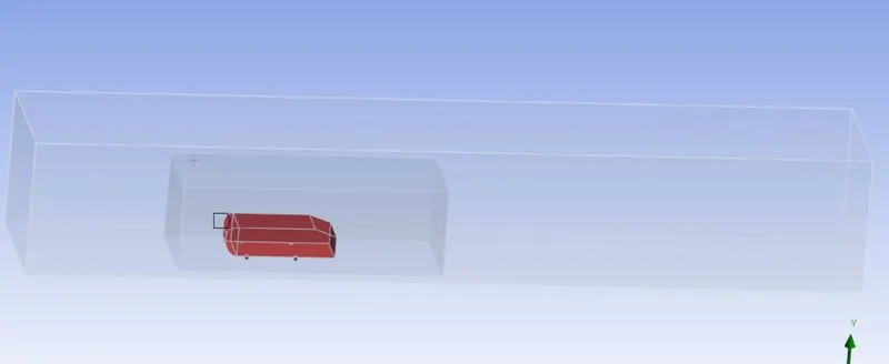
Named sections of domain:

Inlet:

Outlet:

Car-wall:

Symmetry-wall:

Step3: Pre-processing and solver setting

The next step in the simulation after generating the meshing is to set-up the physical properties for the case.

• Type of solver: Density-based
• Simulation method: Steady-state simulation
• Turbulent Model: k-epsilon standard
• Material properties of fluid (Air)

Density: 1.225 kg/m3

Cp (Specific heat): 1006.43 J/kg-k

Thermal Conductivity: 0.0242 w/m-k

Viscosity: 1.7894e-05 kg/m-s

• Inlet velocity: 25 m/s
• Inlet Temperature: 300 K
• Outlet: Pressure type, 0-gauge pressure.
• Walls: wall type with no-slip

Step4 : Expected Results:

1. Velocity and pressure contours.

2. The drag coefficient plot for a refined case. ( For velocity of 25m/sec )

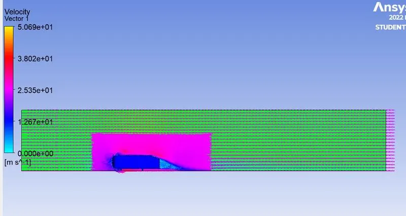
3. The vector plot clearly showing the wake region.

4. Perform the grid independency test and provide the values of drag and lift with each case.

The Following are the various details of the mesh used in this simulation run :

Meshing type	Method	Body sizing	Face sizing	Inflation	Cell count
Baseline	...........	...........	...........	........	84073
1st refinement k-epislon model	Multi zone(70mm)	Inner enclosure(35mm)	Holes(4mm)	First layer thickness=0.7mm and number of layers=10	464599
2nd refinement k-omega model	Multi zone(70mm)	Inner enclosure(35mm)	Holes(4mm)	First layer thickness=0.04mm and number of layers=9	493195

NOTE : Further refinement cannot be done because the cell count exceeds 500000 cells which cannot be solved in the academic version.

Baseline setup results

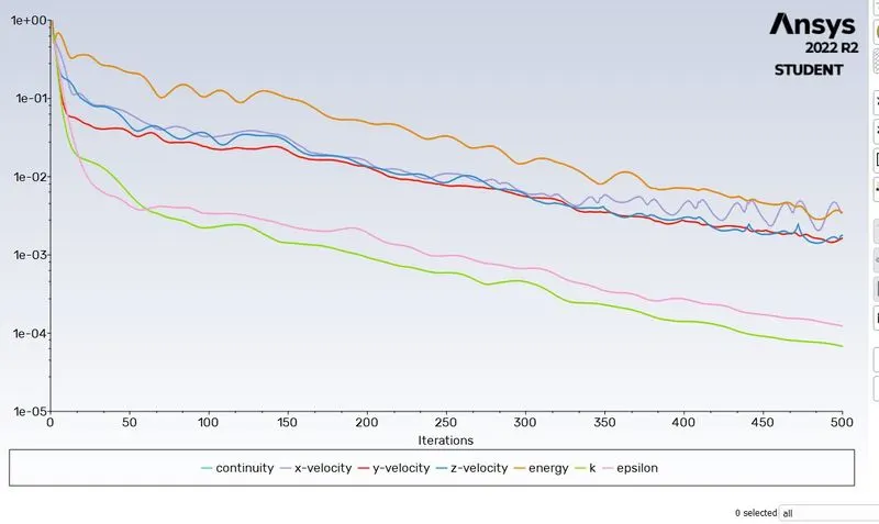
Residual plots:

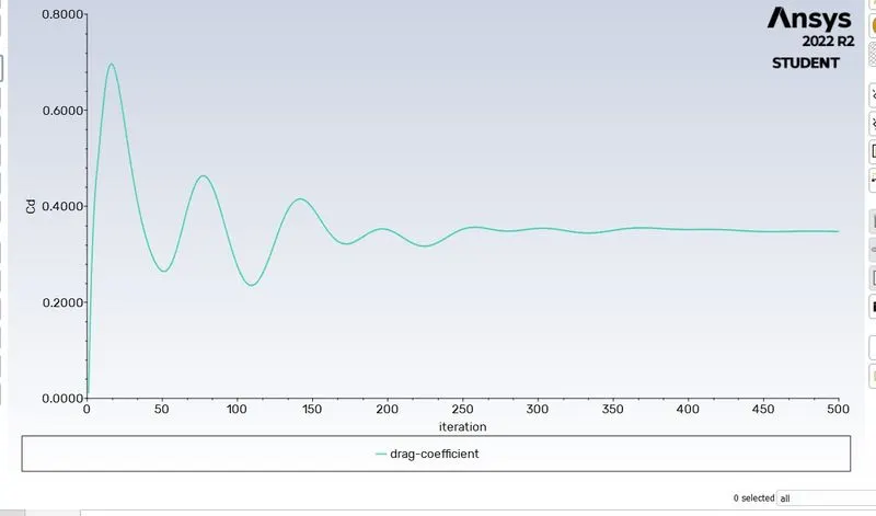
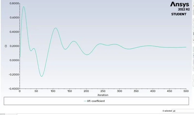
Coefficient of drage and lift:

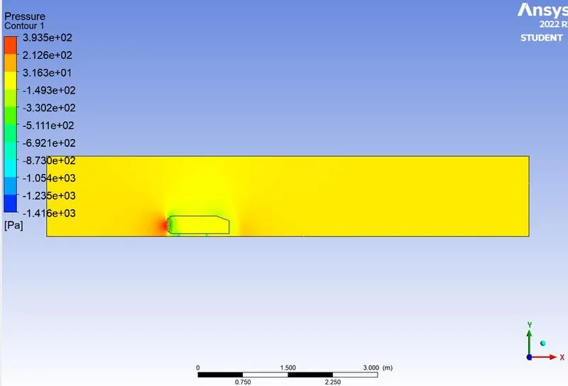
Pressure contour:

Velocity contour:

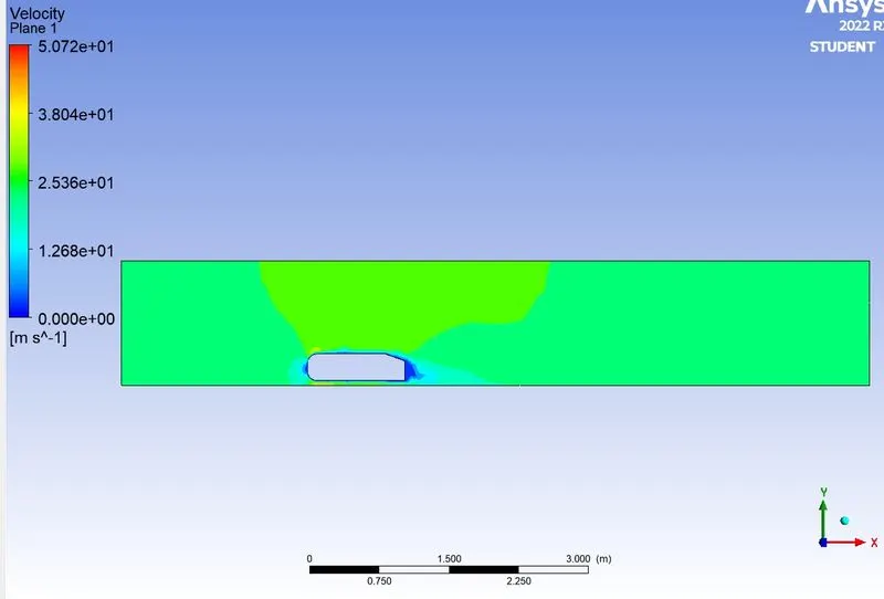
Most refined mesh results(Case-2)

Model:K-epislon

`Y^+=50`

First layer thickness=0.7mm

Number of inflation layers=10

Residual plot:

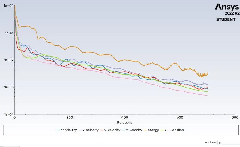
Coefficient of drag and lift:

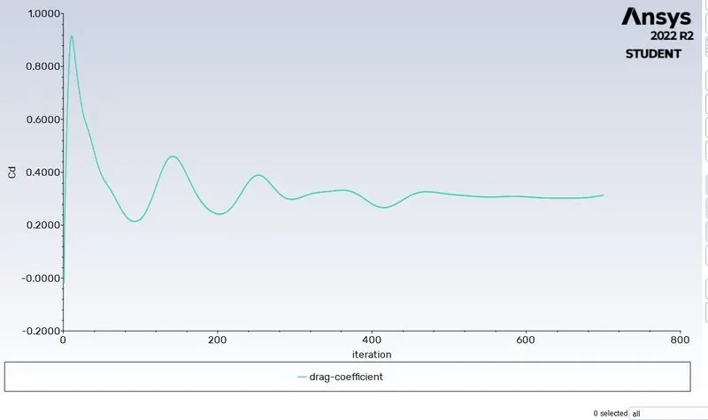
P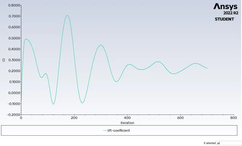

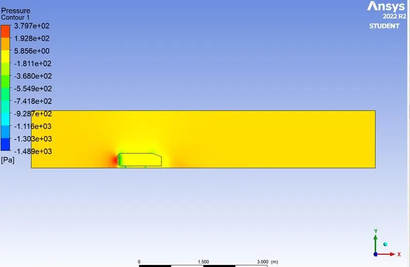
Pressure contour:

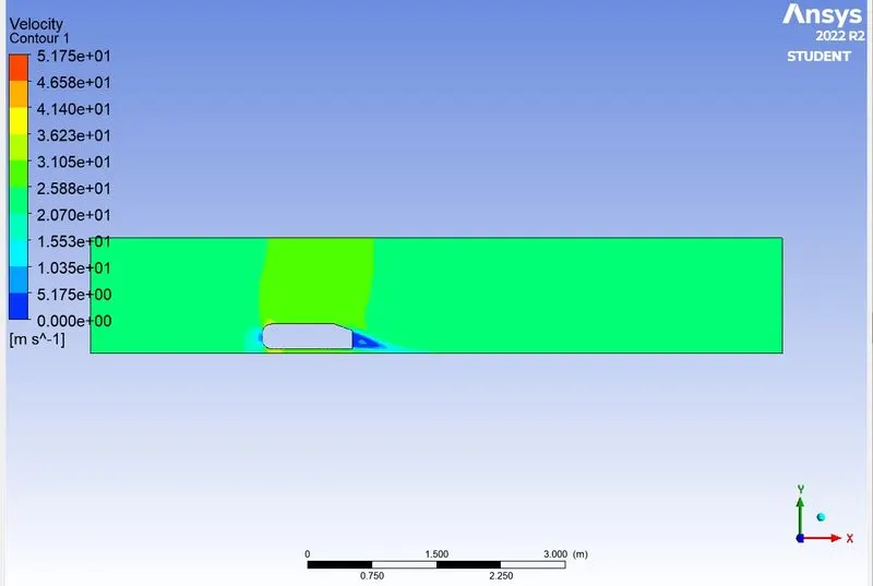
Velocity contour:

Most refined mesh results(Case-3)

Model:K-omega

`Y^+=3`

First layer thickness=0.04mm

Number of inflation layers=9

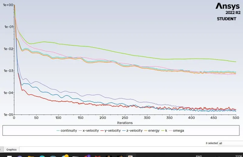
Residual plot:

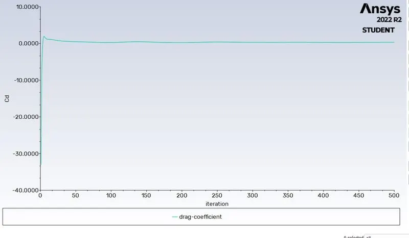
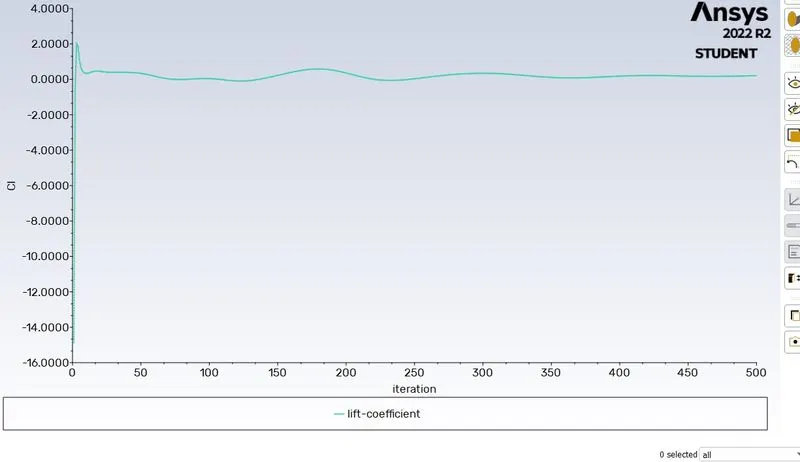
Coefficient of drag and lift:

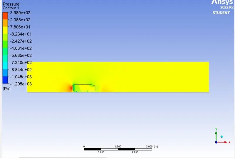
Pressure contour:

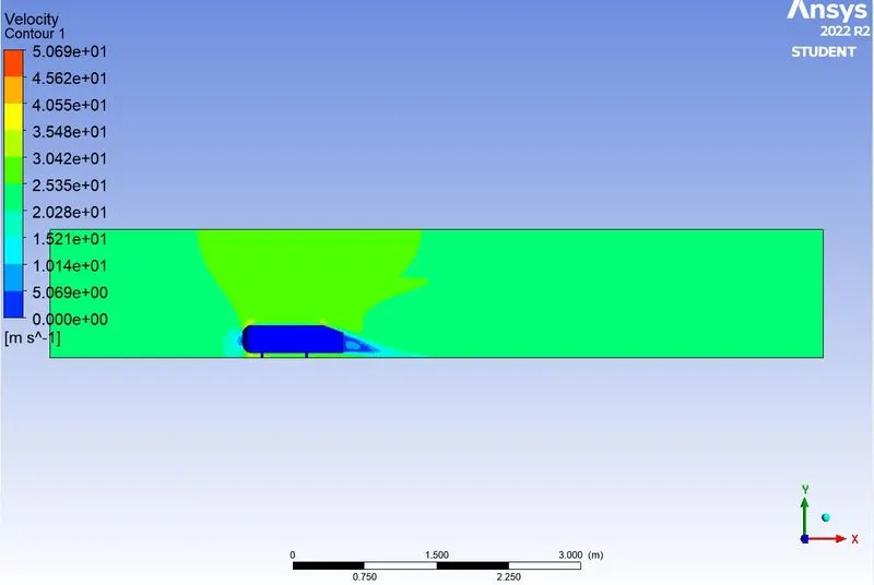
Velocity contour:

Vector plots showing the wake region for most Refined cases:

K-epislon model:

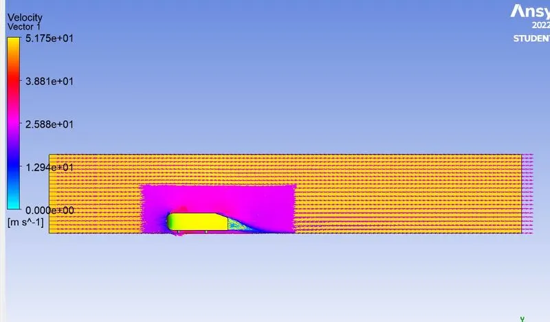
K-omega model:

GRID INDEPENDENCY TEST :

Following table shows the tends of Drag Coefficient vs Refinement :

Mesh type	Drag coefficient	Lift coefficient
Baseline mesh(Refinement=0)	0.34735	0.1845
Refined mesh using k-epislon model	0.31271	0.22452
Refined mesh using k-omega model	0.31520	0.20784

Drag Coefficient :

In fluid dynamics, the drag coefficient is a dimensionless quantity that is used to quantify the drag or resistance of an object in a fluid environment, such as air or water. It is used in the drag equation in which a lower drag coefficient indicates the object will have less aerodynamic or hydrodynamic drag. The drag coefficient is always associated with a particular surface area.

Negative -ve Pressure at Wake :

The moment the flow hits the front of the pressure gets increased , then accordings to Bernoulli’s theorem that flow gets divided between the upstream and downstream of Ahmed body having high and low velocity respectively.

As the flow gets unable to navigate the surface , the upper layer i.e free velocity goes straight . The boundary layer experience a disruption making some of particle get goes straight some gets separated and takes reverse direction , only few particles cope up with contour of the body . this creates a low pressure region that has negative pressure at the back.

On the other hand at the base side , the pressure is high compared to the overhead side of Ahmed body but the pressure keeps on increasing as it can seem to from the contour . The already created low pressure region by the upstream flow causes the flow to move straight.

The pressure region also causes the some air molecules to get reattached to the Ahmed body which makes a recirculation region . The low pressure region at the rear cause a pressure drag . As the flow from the front get heavily attracted gets attracted toward low pressure.

Significance of the Point of Separation :

• A flow separates as soon as it detaches from a surface into a wake . It occurs when the flow slows and there is an increase in the pressure after passing a bluff or streamlined body.

• The position at which the boundary layer leaves the surface of a solid body. It may occur with the laminar flow (laminar separation) or when the boundary layer is turbulent (turbulent separation). Separation is sometimes followed by reattachment of the flow.

• Flow separation or boundary layer separation is the detachment of a boundary layer from a surface into a wake.Separation occurs in flow that is slowing down, with pressure increasing, after passing the thickest part of a streamline body or passing through a widening passage. For example , Flowing against an increasing pressure is known as flowing in an adverse pressure gradient.

Conclusion

After performing numerous simulations on Ahmed body with different meshing parameters, we can draw a few conclusions from this study of CFD simulations.

1) As we refined the meshing, the results are more accurate and clearly showing the wake region behind the Ahmed Body.

2) The negative pressure in a wake region with an increase in velocity is because the Ahmed body is a bluff body. The boundary separation and recirculating of the flow and also the effect of shear stress. To overcome this stress, the pressure turns negative for the balancing effect.

3) Flow separation occurs when the fluid boundary layer encounters an adverse pressure gradient. The point on the body where the boundary layer lifts off the surface is called the separation point. When the airflow separates off the surface, the pressure drag usually increases. To have better performance of an Automobile or any vehicles this separation needs to be avoided or delayed, for smooth flow over the surface of the vehicle.