Week - 3 Drop test Challenge

Week 3: Drop test Challenge

Aim

To develop a detailed simulation file for a drop test, utilize the given nodes and elements of a simplified cellphone model and a plate that represents the ground.

Objectives

Below are the objectives for the challenge.

1. Develop a simulation environment with a simplified cellphone and a plate mimicking the ground. The environment should be set up to perform a drop test.
   
   
2. Use the INITIAL_VELOCITY card to provide velocity specifications for the cellphone. The magnitude of the velocity should be appropriate for simulating a drop test.
   
   
3. Orient the cell phone like its length is perpendicular to the impacting surface. This orientation should be maintained throughout the simulation.
   
   
4. Create a complete input file for the drop test. This file should include all necessary parameters and settings for the simulation.
   
   
5. The simulation should focus on the moment of impact and the few milliseconds following it. The travel of the phone from the hand to the plate is not of interest in this assignment.
   
   
6. The simulation results should be analyzed to understand the behaviour of the cellphone upon impact.
   
   a) The phone bounces back along with rotation after the impact.
   b) The phone bounces back in the same direction after the impact.
   
   
   

Procedure

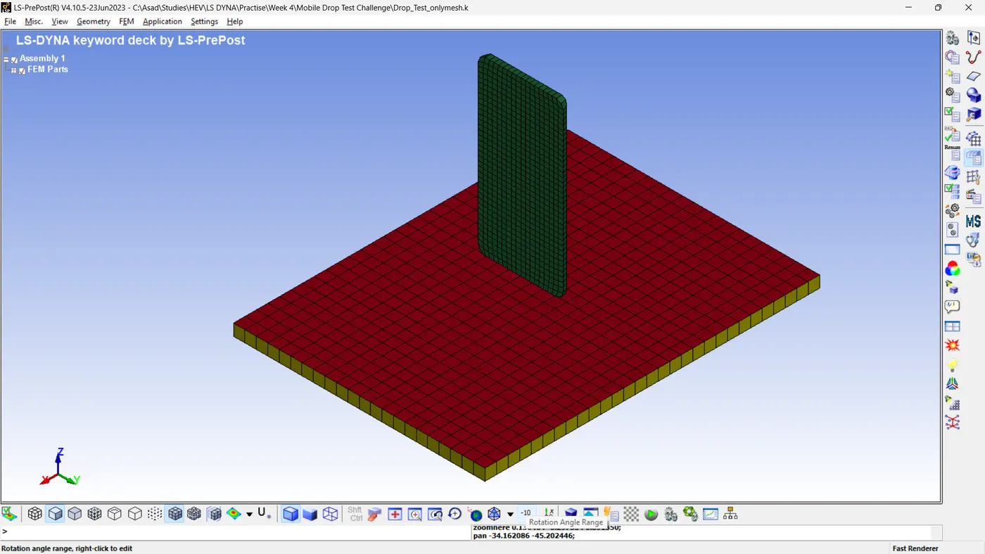
Step 1: Import the model into LS-PrePost.

Download the keyword file and save it in a suitable location. Open LS-Prepost and load the keyword file (.K format).

• File >> Open >> LS-DYNA Keyword File >> Select The File >> Open.
  
  

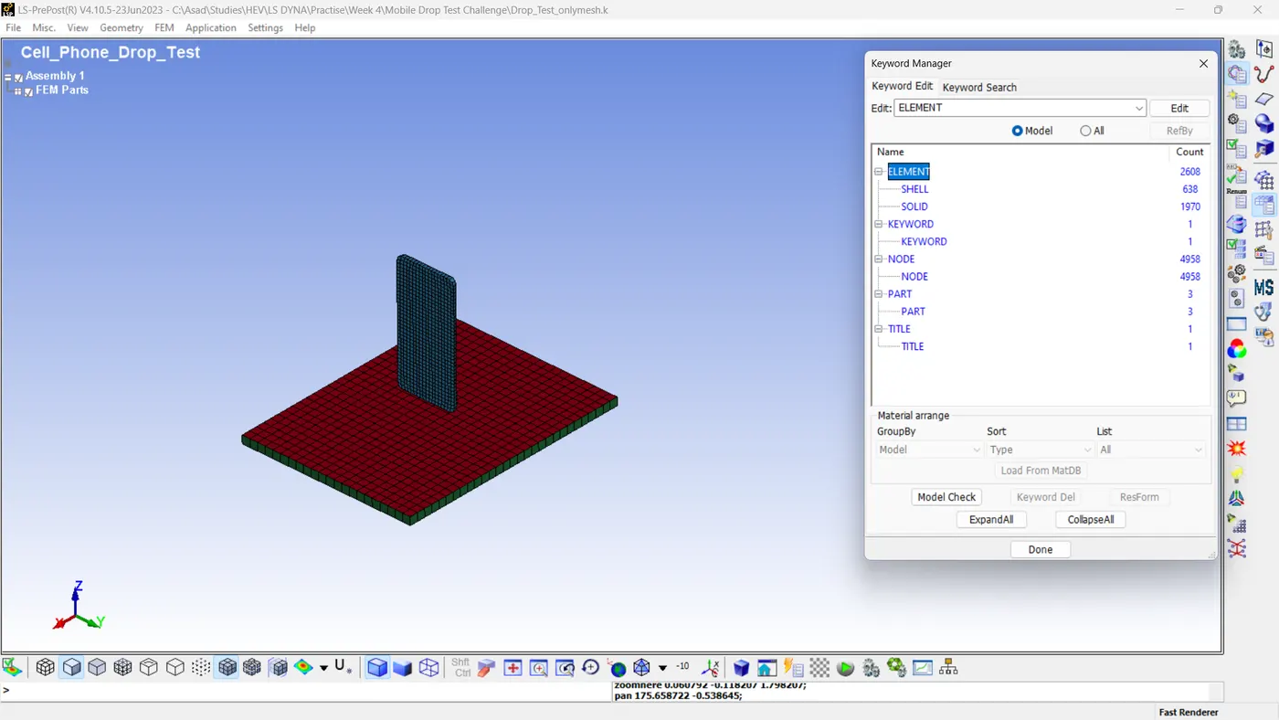
• Model And Part >> Keyword Manager

The keyword manager allows us to identify the existing keywords within the model. With this tool, we can perform minor modifications before the actual setting, such as altering the model name or updating the part name and its PID number.

Step 2: Setting Boundary Conditions.

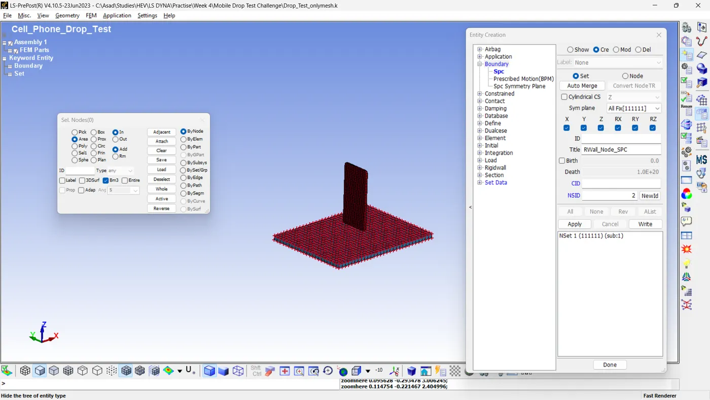
Subsequently, we must impose boundary conditions on the model. Initially, this involves restricting motion in all directions for the wall by fixing the corresponding nodes of specific components. The wall is represented by two parts: one is composed of shell elements, and the other, made of solid elements, lies beneath it.

• Model And Part >> Create Entity >> Boundary >> SPC >> Cre >> Set >> Using Area > Bynode Selection, Select All The Nodes In PID 2 and 3 >> Mark All Six DOFs (X, Y, Z, RX, RY and RZ) >> Give Suitable Title >> Give NSID (Node Set ID) >> Apply >> Done.

Step 3: Assigning Initial Velocity.

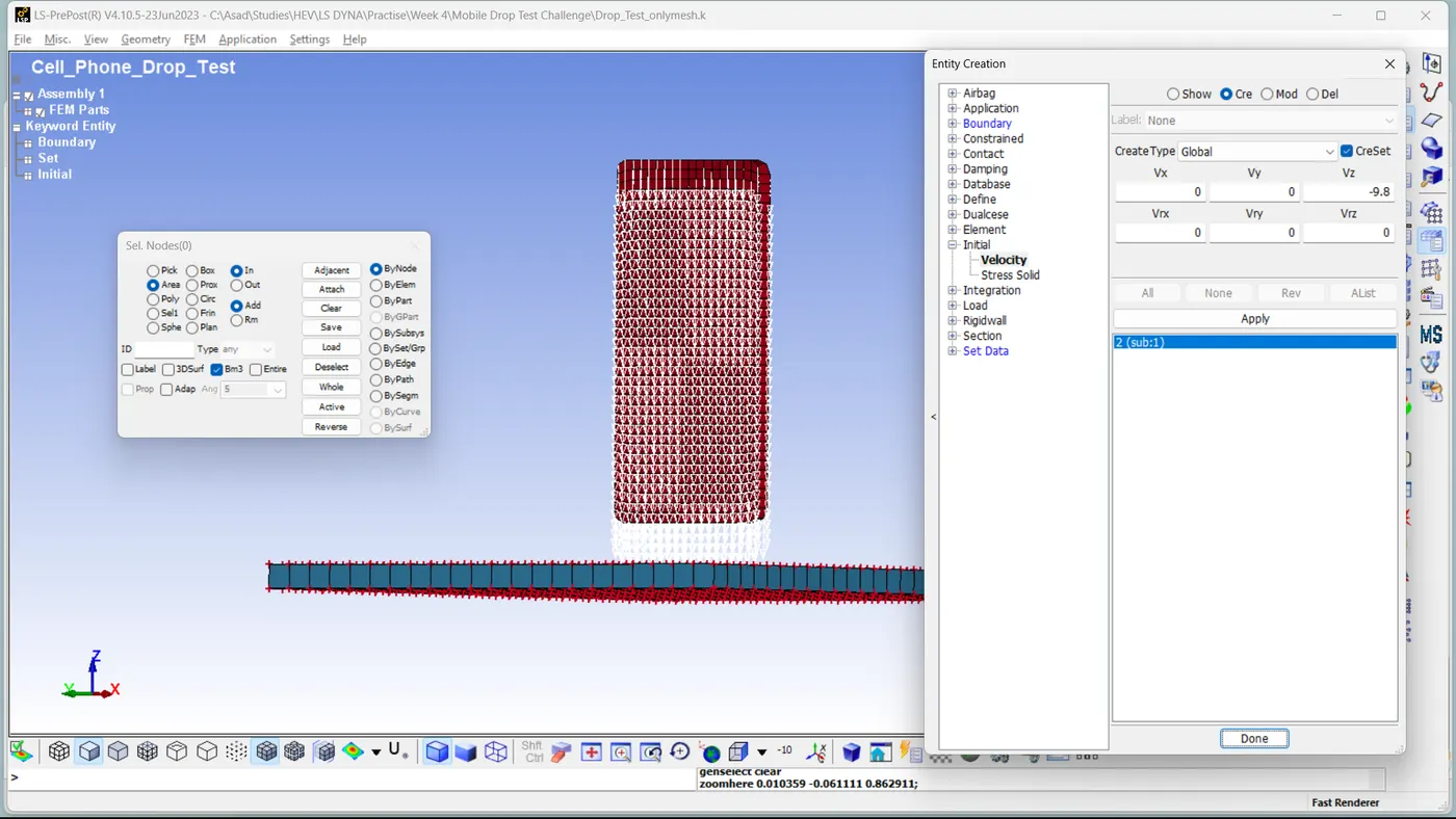
Considering the question, the phone is in a state of free fall. Therefore, the components of the cell phone are moving at a velocity of 9.8 m/s in the direction opposite to the z-axis. Please consider the unit system before inputting the initial velocity values. The initial velocity must be added in mm/ms unit (9.8 m/s = 9.8 mm/ms).

• Model And Part >> Create Entity >> Initial >> Velocity >> Cre >> Mark CreSet >> Using Area > Bynode Selection, Select All The Nodes In PID 1 >> Vz = -9.8, all other velocity values (Vx, Vy, Vrx, Vry and Vrz) is equal to zero >> Apply >> Done

Step 4: Creating Sections.

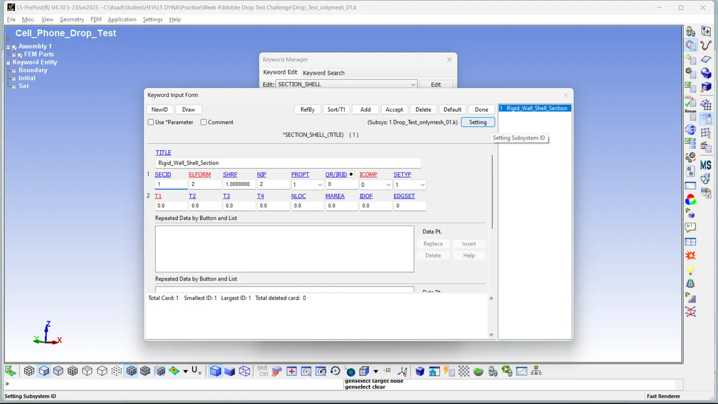
Creating sections will help us determine the internal forces acting on the member. We need to create two sections: one for the shell part and another for the solid part. To create the shell section with default values,

• Model And Part >> Keyword Manager >> All >> Section >> Shell >> Give Suitable Title >> SECID = 1, Maintain other values at their default settings >> Accept >> Done.

To create the solid section with default values,

• Model And Part >> Keyword Manager >> All >> Section >> Solid >> Give Suitable Title >> SECID = 2, Maintain other values at their default settings >> Accept >> Done.

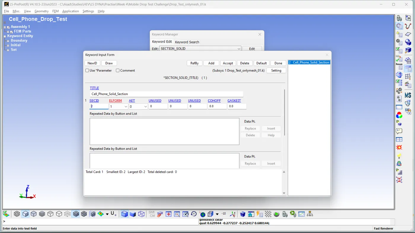
Similarly, create a solid section for the part Rigid_Wall_Solid.

Step 5: Define Material.

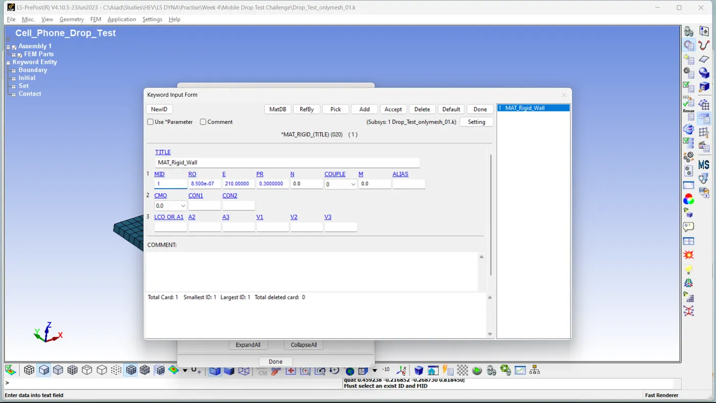
Each part needs its material definition. Here the Wall component is defined with MAT_020 (Rigid). The material definition for the wall component, along with the values for the required parameters, is as follows:

1. RO = 850 Kg/m^3 = 850 x10^-9 Kg/mm^3
   
   
2. E = 210 GPa = 210 Kg/mm ms^2
   
   
3. PR = 0.3

• Model And Part >> Keyword Manager >> All >> MAT >> 020-Rigid >> Give Suitable Title >> MID =1, RO = 850 x 10^-9 Kg/mm^3, E = 210 Kg/mm mms^2, PR = 0.3, Maintain other values at their default settings >> Accept >> Done.

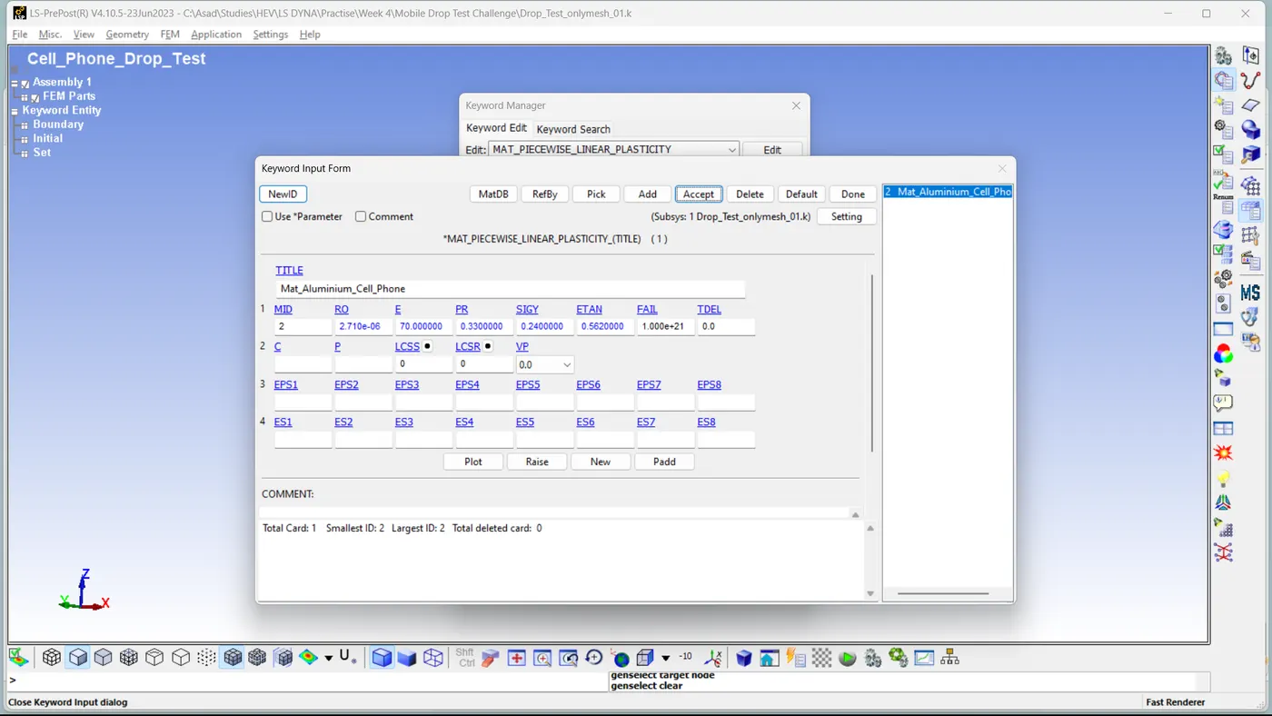
For defining the cell phone, we can rely on MAT-24 (Mat_Piecewise_Linear_Plasticity). For the parameter data, we can consider the material as made of Aluminium. The material definition for the wall component, along with the values for the required parameters, is as follows:

1. RO = 2710 Kg/m^3 = 2710 x10^-9 Kg/mm^3
   
   
2. E = 70 GPa = 70 Kg/mm ms^2
   
   
3. PR = 0.33
   
   
4. SIGY = 240 MPa = 0.240 Kg/mm ms^2
   
   
5. ETAN = 562 MPa = 0.562 Kg/mm ms^2

• Model And Part >> Keyword Manager >> All >> MAT >> 024-Piecewise_Linear_Plasticity >> Give Suitable Title >> MID =2, RO = 2710 x 10^-9 Kg/mm^3, E = 70 Kg/mm mms^2, PR = 0.33, SIGY = 0.240 Kg/mm ms^2 and ETAN = 0.562 Kg/mm ms^2. Maintain other values at their default settings >> Accept >> Done.

Step 6: Assigning Sections And Material To Parts.

For the cellphone component, we must allocate a solid section and designate it as MAT-024. To accomplish this,

• Model And Part >> Keyword Manager >> Model >> Part >> Cell Phone >> Select MID = 2 (For MAT-24) >> Select SECID = 2 (For Cell_Phone Solid Section) >> Maintain other values at their default settings >> Accept >> Done.
  
  

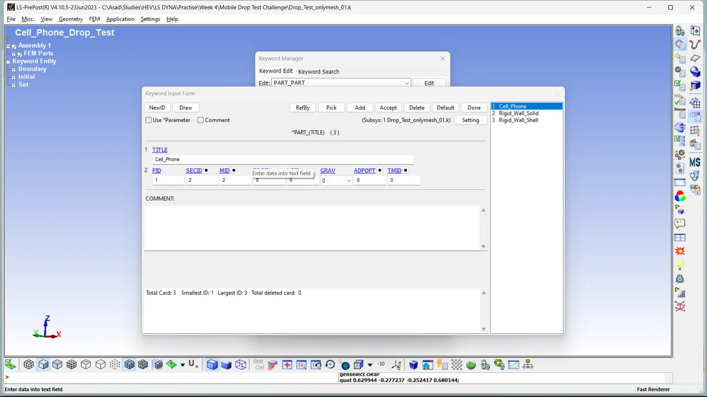
For the Rigid_Wall_Shell component, we must allocate a shell section and designate it as MAT-020. To accomplish this,

• Model And Part >> Keyword Manager >> Model >> Part >> Rigid_Wall_Shell >> Select MID = 1 (For MAT-20) >> Select SECID = 1 (For Rigid_Wall_Shell_Section) >> Maintain other values at their default settings >> Accept >> Done.

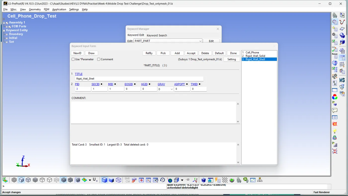
Because of the Rigid_Wall_Shell part, the Rigid_Wall_Solid does not affect the simulation. The shell part is a rigid wall and its motions are constrained in every direction. So no cell phone element can penetrate the shell surface. However, we must also assign a section and material to that part to prevent errors in the simulations.

Step 7: Defining Contacts.

This analysis identifies two types of contacts. The first is the contact between the cell phone and the rigid wall shell surface, and the second is the self-contact occurring among the cell phone's elements. The contact between the cell phone and the rigid wall shell surface is defined by,

• Model And Part >> Keyword Manager >> All >> Contact >> Automatic_Surface_To_Surface >> Give Suitable Title >> CID =1 >> SURFATYP = 3 (For Selecting Part ID as Slave) >> SURFBTYP = 3 (For Selecting Part ID as Master) >> SURFA = 1 (Part ID Of Cell Phone As Slave) >> SURFB = 3 (Part ID Of Rigid_Wall_Shell As Master) >> Maintain other values at their default settings >> Accept >> Done.

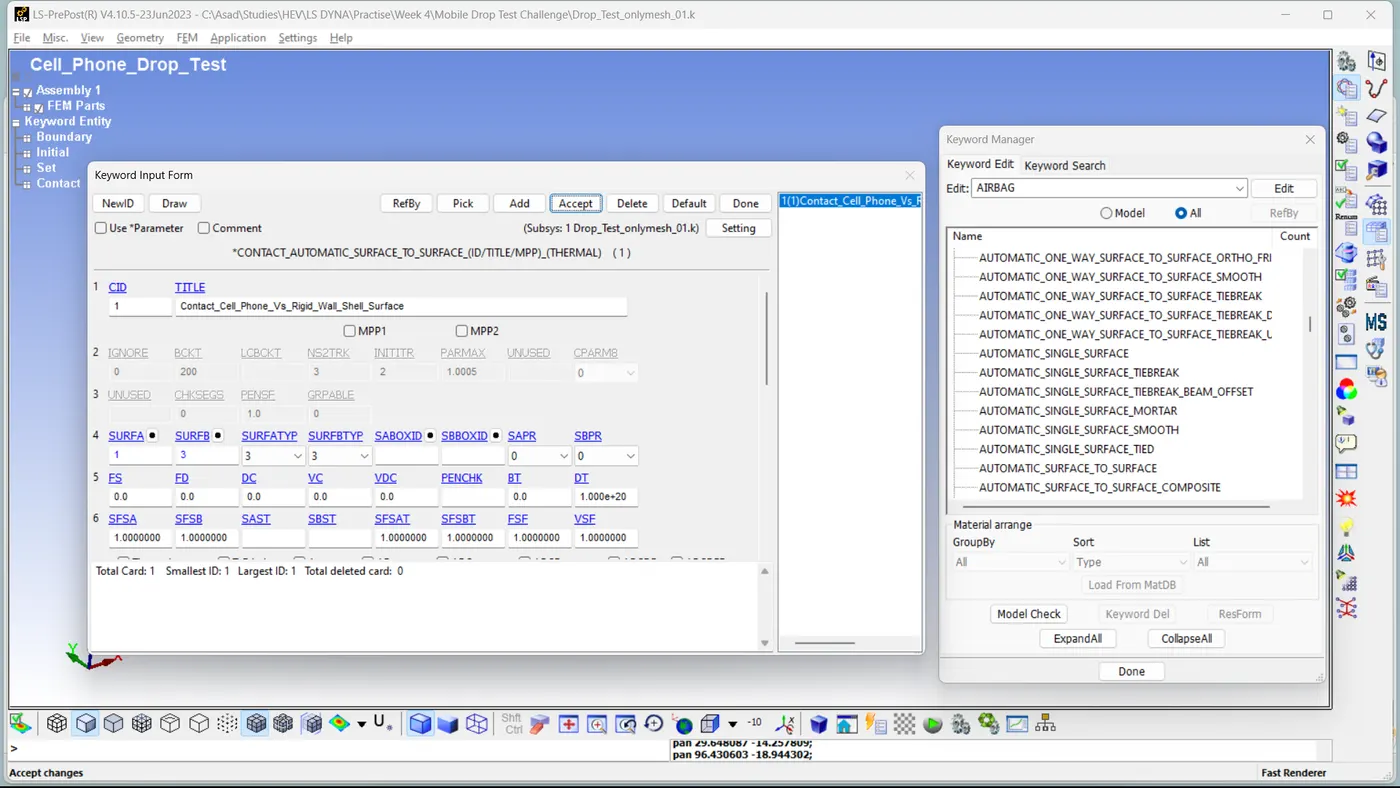
The self-contact occurring among the cell phone's elements is defined by,

• Model And Part >> Keyword Manager >> All >> Contact >> Automatic_Single_Surface >> Give Suitable Title >> CID =2 >> SURFATYP = 3 (For Selecting Part ID as Slave) >> SURFBTYP = 0 (Not Applicable For Self Contact) >> SURFA = 1 (Part ID Of Cell Phone As Slave) >> SURFB = 0 (Not Applicable For Self Contact) >> Maintain other values at their default settings >> Accept >> Done.

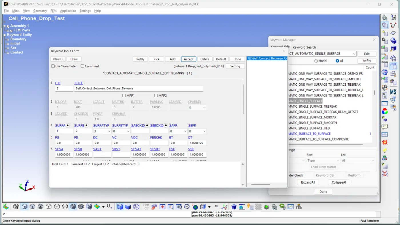
Step 8: Defining Control Cards.

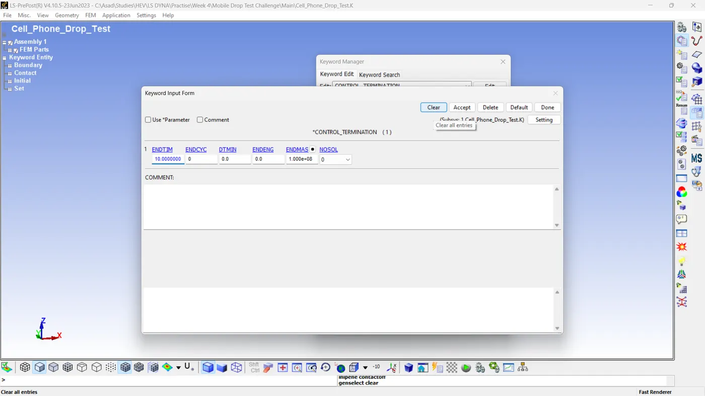
We can define the control card for the termination. For that,

• Model And Part >> Keyword Manager >> All >> Control >> Termination >> ENDTIM =10 >> Maintain other values at their default settings >> Accept >> Done.

Step 9: Setting Data Bases.

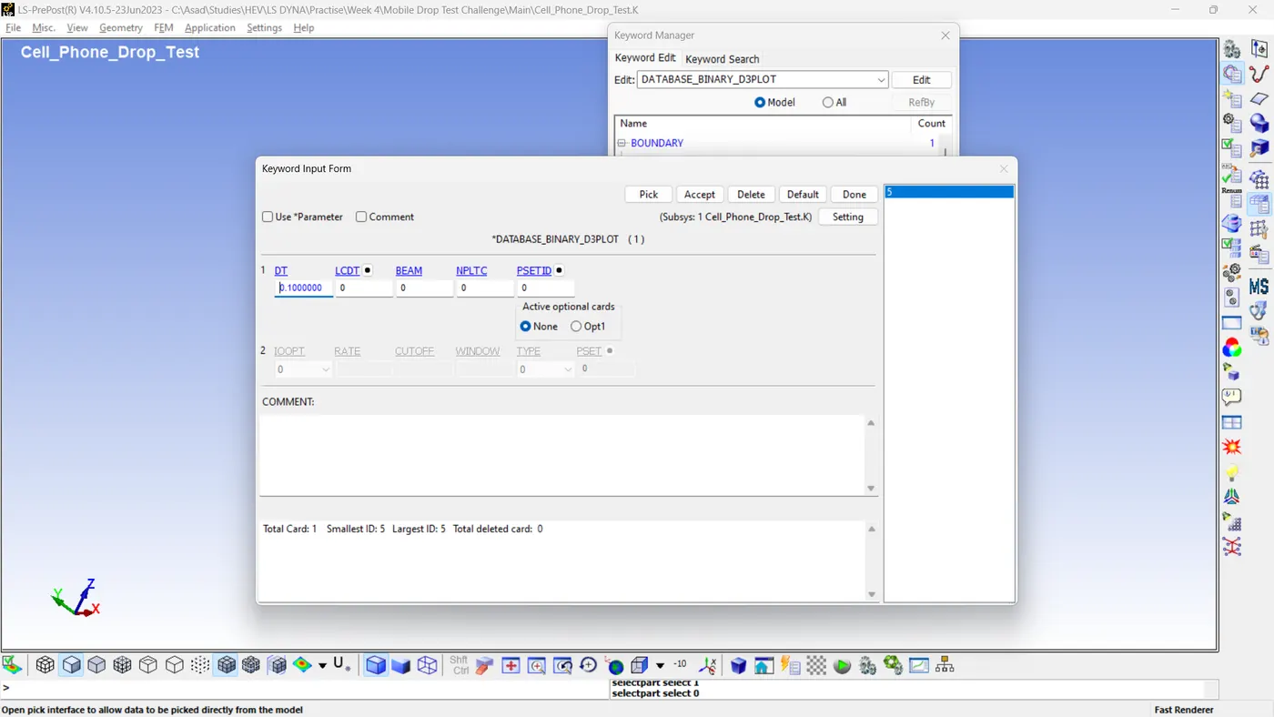
For binary outputs, the only one required is 'Binary_D3PLOT'. It is used for the complete output stats. To activate that,

• Model And Part >> Keyword Manager >> All >> Database >> Binary_D3PLOT >> DT=0.1 >> Maintain other values at their default settings >> Accept >> Done.

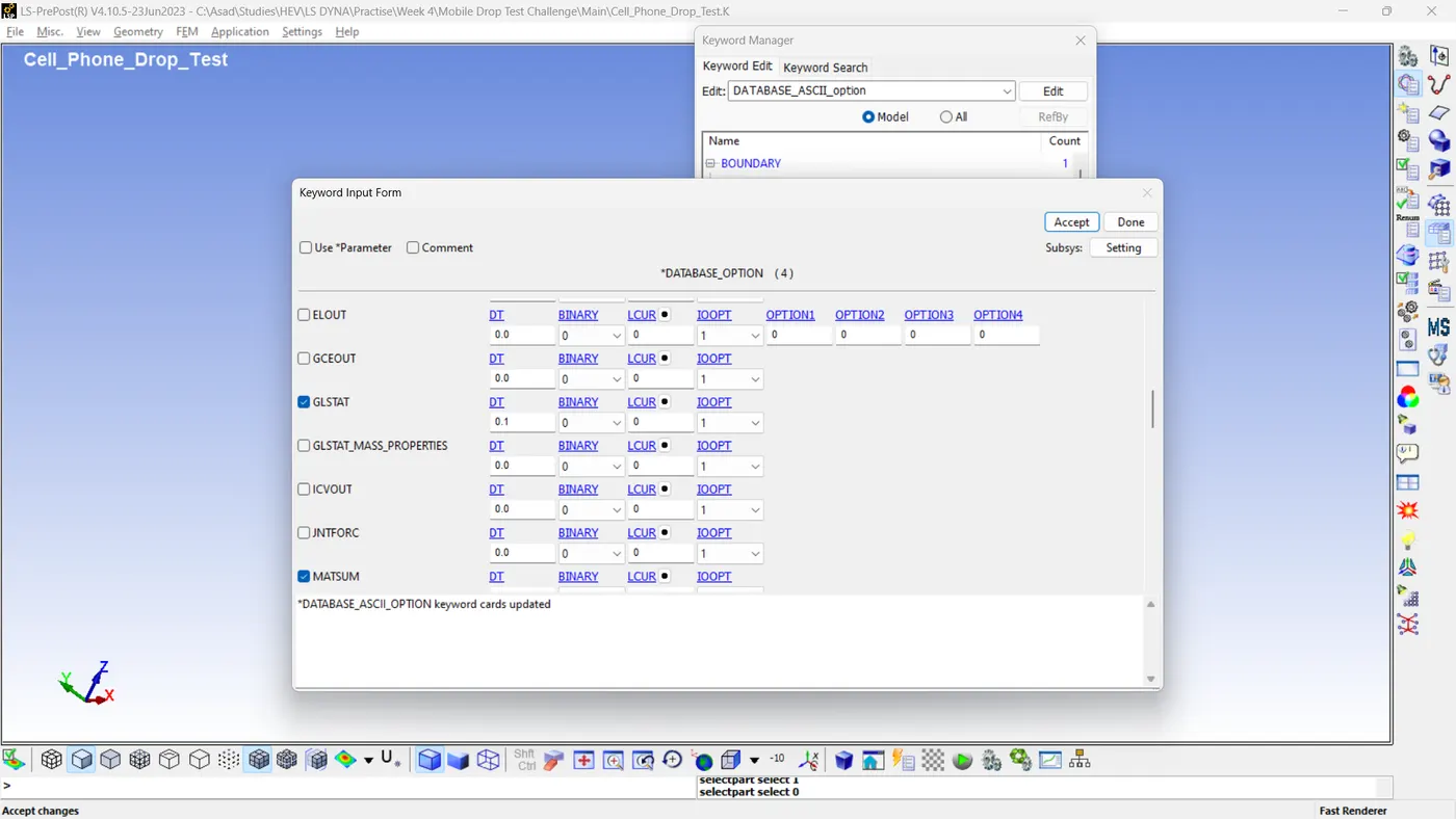
For ASCII outputs, we need the following cards

1. GLSTAT (Global Data / All Energy Data)
   
   
2. MATSUM (Material Energies Part By Part)
   
   
3. RCFORC (Resultant Interface Force)
   
   
4. SECFORC (Cross Sectional Force)

To activate those databases,

• Model And Part >> Keyword Manager >> All >> Database >> ASCII_Option >>Select The Database Cards >> DT=0.1 >> Maintain other values at their default settings >> Accept >> Done.

Step 10: Model Checking And Final Model.

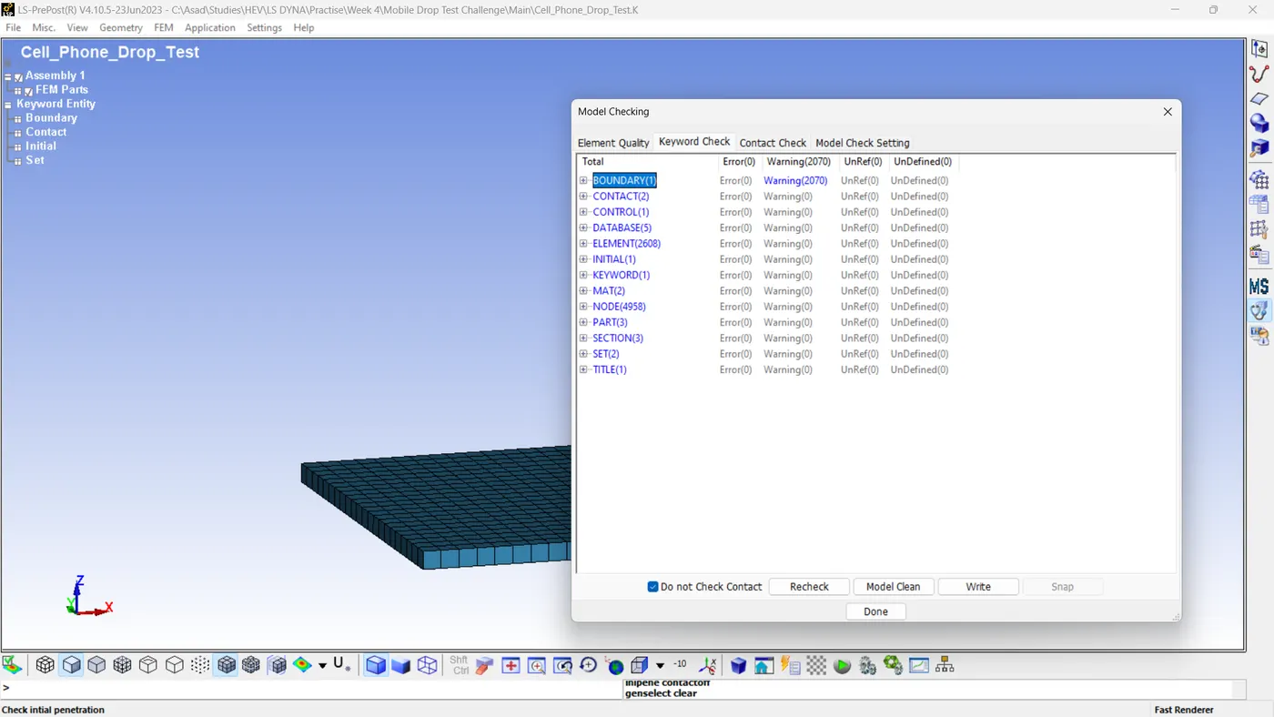
Model checking can be used for finding errors in the model, It can be done by

• Model And Part >> Keyword Manager >> Model Check >> Review Results >> Done

Step 11: Running The Simulation And Loading The Simulation.

To run the simulation, we need to save the file with the '.K' extension. Then,

• File >> Run LS-DYNA >> Browse The File Location >> Run.

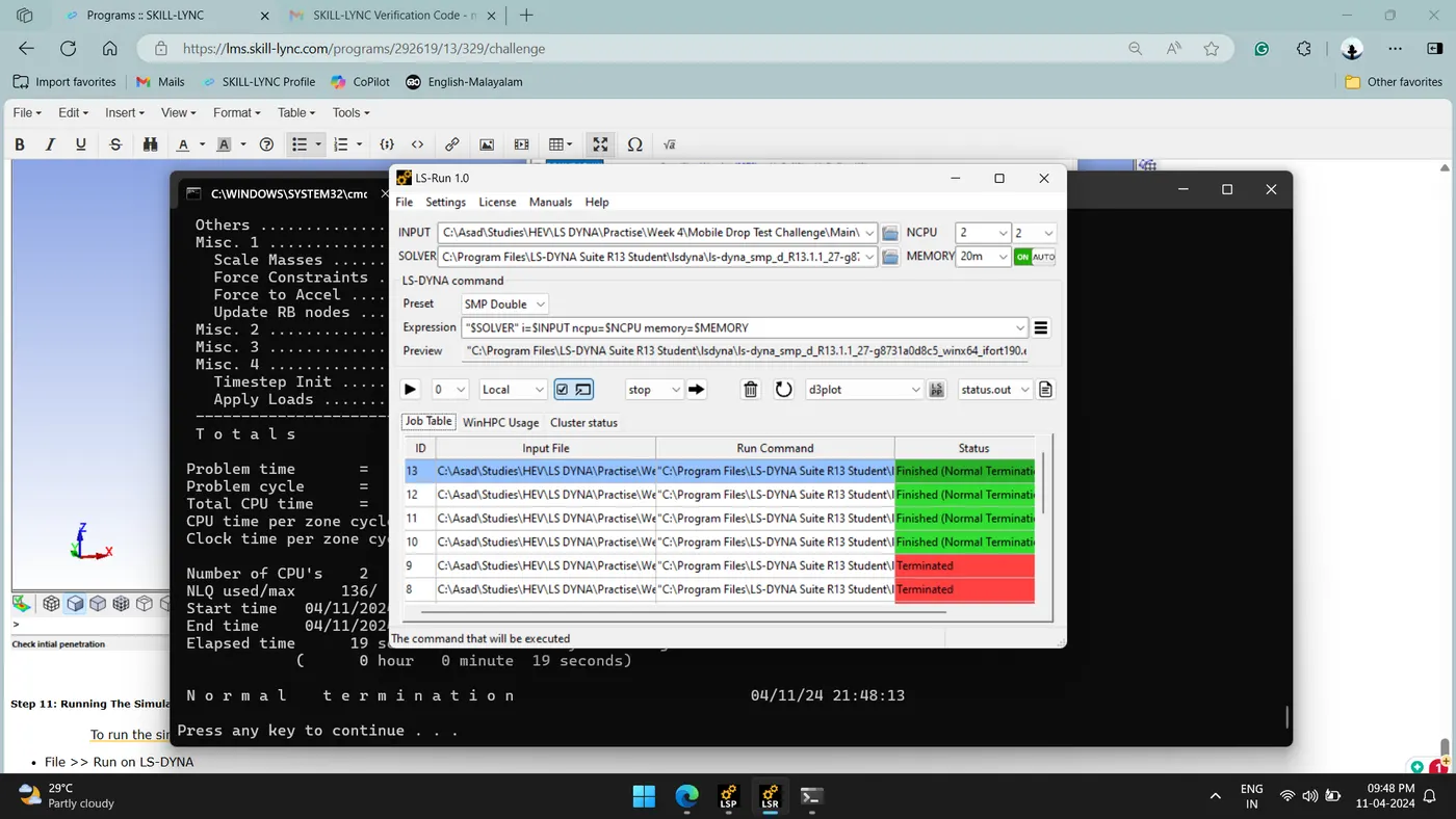
After successful termination, the necessary files, including the binary file, are saved in the desired location. We can load them by,

• File >> Open >> LS-DYNA Binary Plot >> Select The D3PLOT File >> Open.

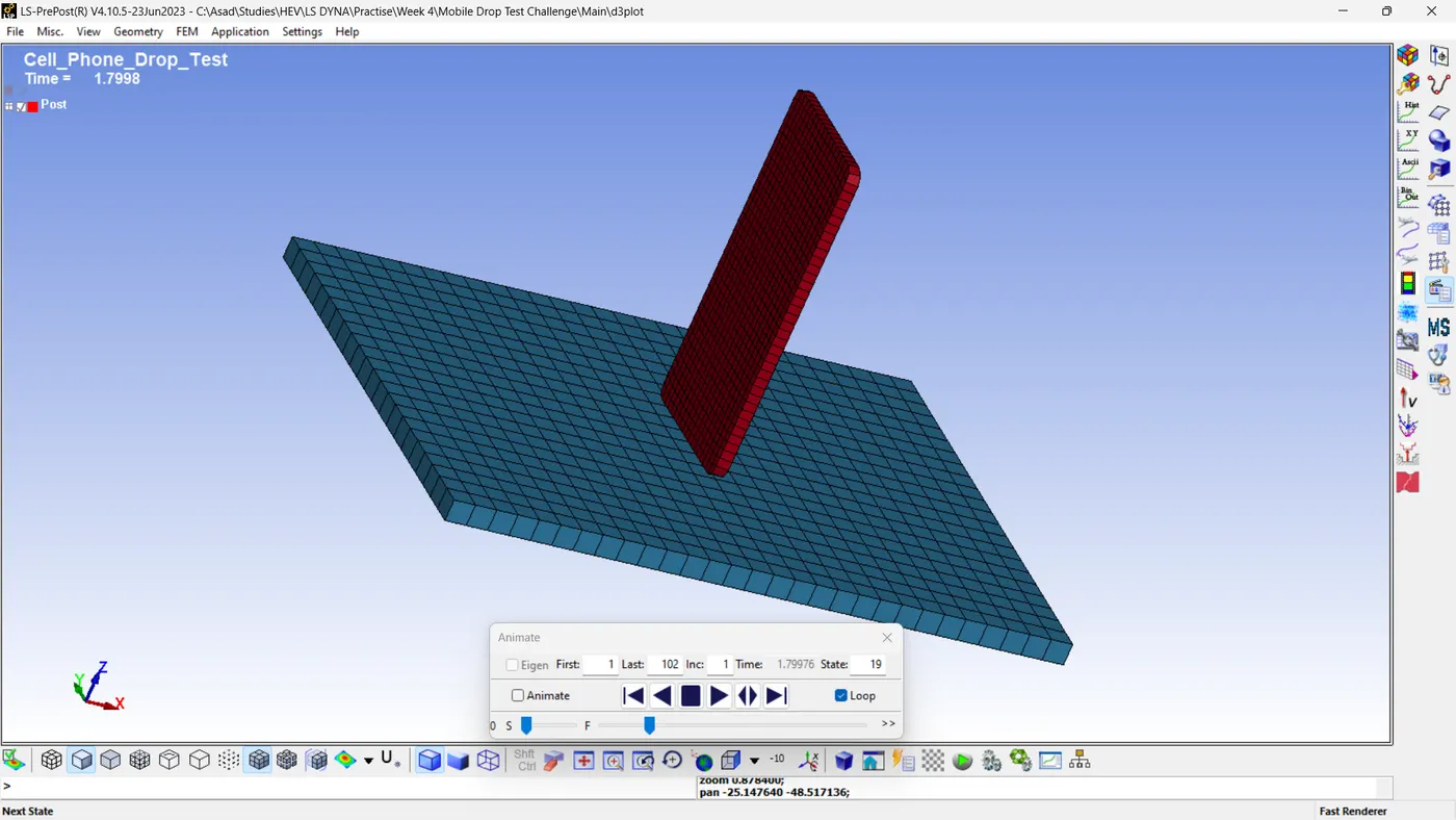
We can execute the simulation and analyze the outcomes by utilising the action controls.

Step 12: Plotting The Results.

1. Von-Mises Stress

To show the effects of von-mises stresses,

• Post >> Fringe Component >> Stress >> Von Mises Stress >> Play Animation >> Analyse The Results.

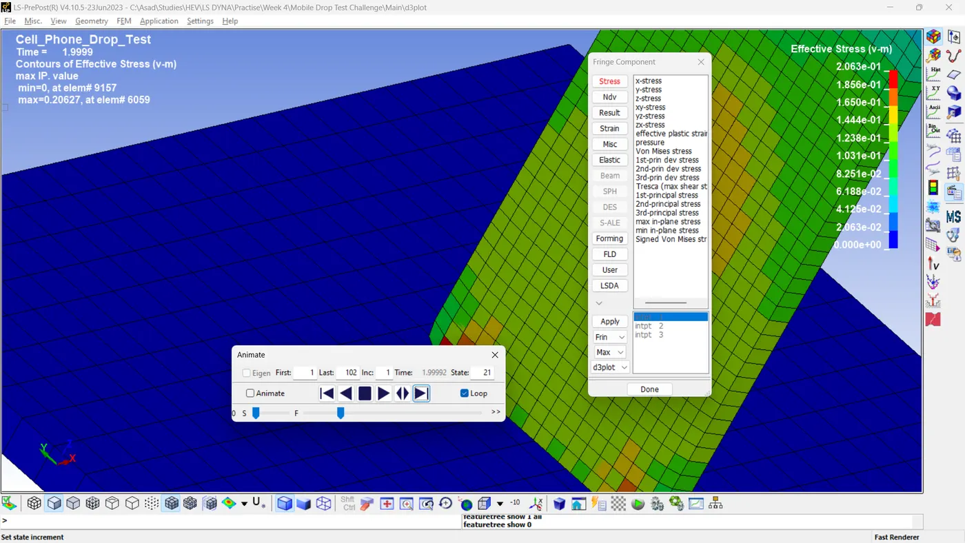
From the results, it is evident that the maximum Von-Mises stress occurs at the initial contact of the cell phone with the rigid surface. The maximum value of Von-Mises Stress = 0.206 kg/mm ms^2 = 206 MPa at 1.999 ms.

2. Kinetic Energy Vs Time

To plot the kinetic energy plot,

• Post >> History >> Global >> Kinetic Energy >> Plot.
  

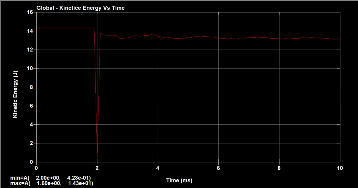
Similarly, we can plot other global energy plots and other necessary plots.

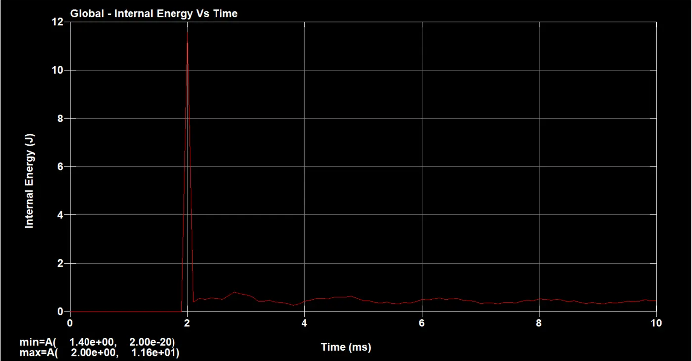
3. Internal Energy Vs Time

4. Total Energy Vs Time

Results And Conclusion

• The simulation is conducted by assigning appropriate materials and sections, and by applying an initial velocity. The changes in global energy values are analyzed using animations and plots. The following results were obtained from the simulation.
  
  1. For the Von-Mises Stress,
  Maximum Value = 206 MPa at 1.999 ms.
  

  2. For the Kinetic energy
  Minimum Value = 0.423 J at 2.0 ms
  
  3. For the Internal energy,
  Maximum Value = 11.6 J at 2.0 ms
  
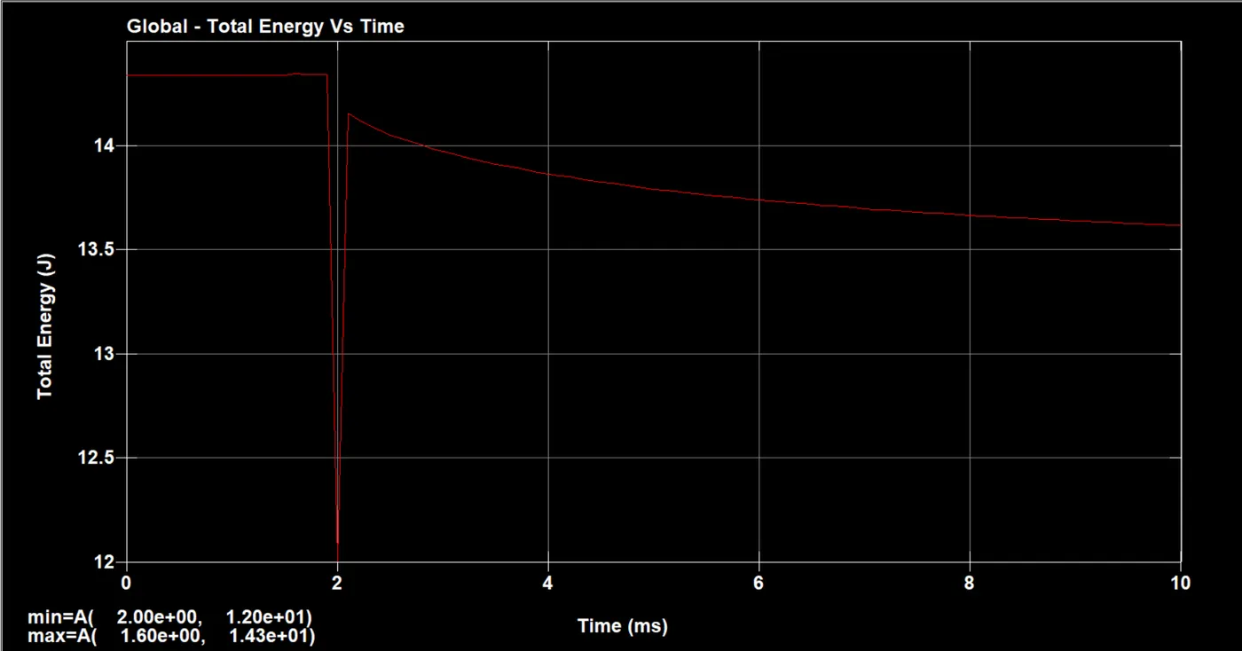
  4. For the Total energy,
  Maximum Value = 14.3 J at 1.6 ms
  Minimum Value = 12.0 J at 2.0 ms
  

• During the simulation, it was observed that the phone bounced back in the same direction from which it fell onto the surface. The phone does not rotate during the simulation. This is because the initial velocity is applied solely in the z-direction. Additionally, the rigid wall lies in the xy-plane, which means it is perpendicular to the z-axis. Thus, the velocity does not induce any rotational effects on the phone.
  
  
• The Von Mises stress reaches its maximum value when the cell phone comes into contact with a surface.
  
  
• Similarly, when the cell phone comes into contact with a surface, its kinetic energy reaches a minimum, its internal energy peaks, and its total energy is at its lowest.
  
  
• In the case of kinetic energy, there is a noticeable decrease in its value upon contact with a surface. The cell phone bounces back, suddenly recovering most of its kinetic energy, and then follows a disruptive pattern until the end of the simulation.
  
  
• In the case of internal energy, there is a noticeable increase in its value upon contact with a surface. The cellphone rebounds, abruptly losing much of its internal energy, and then exhibits a disruptive pattern until the simulation concludes.
  
  
• The aforementioned changes alter the characteristics of total energies. Evidence of energy loss is often observed when surfaces come into contact. This can be attributed to friction or heat dissipation.

Reference

• LS-DYNA_Keyword_Manual_Volume_I_R13
  
• LS-DYNA_Material_Manual_Volume_II_R13
  

G-Drive Link

https://drive.google.com/drive/folders/1iVctuBaQgjovObqU7ouFtoBnUyLlsNUE?usp=sharing