Python&Cantera - Adiabatic Flame Temperature calculation
Aim: Calculating adiabatic flame temperature (AFT) using Python and Cantera
Objective:
- Obtain trend for AFT vs equivalence ratio
- AFT of combustion of methane in presence of heat loss (heat loss = 0.35)
- AFT comparison for general alkanes
- AFT comparison for 2 carbon atom species
Theory:
AFT represents total energy input into a furnace for specific fuel rate and combustion stoichiometry, and thus is generally used as a design criterion for air-firing combustion chambers. The adiabatic flame temperature is one that occurs when the combustion chamber is well insulated with no heat losses (adiabatic conditions). The peak adiabatic flame temperature occurs at around equivalence ratio of 1, in an ideally insulated combustion chamber.
In study of combustion, there are two types of adiabtic flame temperatures, depending on how the process is completed; constant volume and constant pressure. The constant volume adiabatic flame temperature is the temperature that results from a complete combustion process that occurs without any work, heat transfer or change in KE or PE. Its temperature is hgher than the constant pressure process because no energy is utilized to change the volume of the system, thus no generation of work.
NASA's Thermodynamic data file contains coefficients for polynomials that are used to calculate thermodynamic properties for various chemical species. Hence, following formulae were developed:
`(Cp)/R = a1 + a2 T + a3 T^2 + a4 T^3 + a5T^4`
`H/(RT) = a1 + (a2T)/2 + (a3 T^2)/3 + (a4 T^3)/4 + (a5 T^4)/5 + (a6)/T`
`S/R = a1 lnT + a2 T + (a3 T^2)/2 + (a4 T^3)/3 + (a5 T^4)/4 +a7`
Newton Raphson Method:
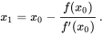
In numerical analysis, Newton-Raphson method (NR method), is a root finding algorithm which produces successively better approximations to the roots (or zeroes) of a real valued function. The most basic version starts with a single variable function `f` defined for a real variable `x`, the function's derivative `f'`, and an initial guess `x0` for a root of `f`. If the function satisfies sufficient assumptions and the intitial guess is close, then
The iterative form is given as
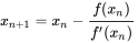
Using the above, we'll code an iterative solver that would calculate AFT by equating enthalpies of the enthalpies of reactants and products in a chemical reaction. The enthalpies are determined by NASA polynomial functions given above.
Stoichiometric `(phi = 1): CH4 + 2(O2 + 3.76N2) <=> CO2 + 2H2O + 7.52N2`
Rich Mixture `(phi > 1): CH4 + (2/phi)(O2 + 3.76N2) <=> (4/phi - 3)CO2 + 2H2O + (7.52/phi)N2 + (4 - 4/phi)CO`
Lean Mixture `(phi < 1): CH4 + (2/phi)(O2 + 3.76N2) <=> CO2 + 2H2O + (7.52/phi)N2 + (2/phi - 2)O2`
Codes:
Case-1: AFT vs Equivalence Ratio
Equialence Ratio is defined as the ratio of sample air-fuel mixture to the stoichiometric air-fuel mixture. Depending on equivalence ratio, a combustion reaction may occur in a controlled way or an explosion.
Here, reaction is occuring in a constant volume combustion chamber, hence, we need to balance enthalpy as well as number of moles of reactants and products.
The products of reaction varies with equivalence ratio (`phi`). A rich mixture has `phi`>1 and a lean mixture has `phi`<1. `phi`=1 signifies that the mixture is as per stoichiometry.
In the code, we import the modules we require (numpy, matplotlib and cantera). Then, NASA polynomial function is defined in a function and the coefficients are provided at later part. This function is then called into a function to calculate enthalpy and moles of reactants and products. The derivative of this function is defined. This is used in the newton raphson iterator. The output i.e. temperature of flame is stored into array. Hence, AFT is obtained by Python. Cantera as built in tools and the results are stored and works by minimizing Gibbs free energy to obtain quilibrium. Comparison between Python and Cantera is drawn by plotting and tabulating the results.
"""
Adiabatic Flame Temperature Using Python and Cantera

Stoichiometric (phi = 1): CH4 + 2(O2 + 3.76N2) <=> CO2 + 2H2O + 7.52N2
Rich Mixture (phi > 1): CH4 + (2/phi)(O2 + 3.76N2) <=> (4/phi - 3)CO2 + 2H2O + (7.52/phi)N2 + (4 - 4/phi)CO
Lean Mixture (phi < 1): CH4 + (2/phi)(O2 + 3.76N2) <=> CO2 + 2H2O + (7.52/phi)N2 + (2/phi - 2)O2

"""
#Importing Required Packages
from matplotlib.pyplot import *
import cantera

"""
Solution Obtainedby Python
"""
R = 8.314	# J/mol-K

# Function to calculate enthalpy of a compound through NASA polynomial function
def h(T, coeff):
	a1 = coeff[0]
	a2 = coeff[1]
	a3 = coeff[2]
	a4 = coeff[3]
	a5 = coeff[4]
	a6 = coeff[5]
	return (a1 + a2*T/2 + a3*pow(T,2)/3 + a4*pow(T,3)/4 + a5*pow(T,4)/5 + a6/T)*R*T

# Coefficients for the NASA polynomial for low temperatures
ch4_coeff_l = [5.14987613E+00, -1.36709788E-02, 4.91800599E-05, -4.84743026E-08, 1.66693956E-11, -1.02466476E+04, -4.64130376E+00]
o2_coeff_l = [3.78245636E+00, -2.99673416E-03, 9.84730201E-06, -9.68129509E-09, 3.24372837E-12, -1.06394356E+03, 3.65767573E+00]
n2_coeff_l = [0.03298677E+02, 0.14082404E-02, -0.03963222E-04, 0.05641515E-07, -0.02444854E-10, -0.10208999E+04, 0.03950372E+02]
# Coefficients for the NASA polynomial for high temperatures
co2_coeff_h = [3.85746029E+00, 4.41437026E-03, -2.21481404E-06, 5.23490188E-10, -4.72084164E-14, -4.87591660E+04, 2.27163806E+00]
h2o_coeff_h = [3.03399249E+00, 2.17691804E-03, -1.64072518E-07, -9.70419870E-11, 1.68200992E-14, -3.00042971E+04, 4.96677010E+00]
n2_coeff_h = [0.02926640E+02, 0.14879768E-02, -0.05684760E-05, 0.10097038E-09, -0.06753351E-13, -0.09227977E+04, 0.05980528E+02]
co_coeff_h = [2.71518561E+00, 2.06252743E-03, -9.98825771E-07, 2.30053008E-10, -2.03647716E-14, -1.41518724E+04, 7.81868772E+00]
o2_coeff_h =  [3.28253784E+00, 1.48308754E-03, -7.57966669E-07, 2.09470555E-10, -2.16717794E-14, -1.08845772E+03, 5.45323129E+00]

# Standard temperature condition
Tstp = 298.15	# K

# Defining the function for root-solving by Newton-Raphson method
def f(T, phi):
	h_ch4_r = h(Tstp, ch4_coeff_l)
	h_o2_r = h(Tstp, o2_coeff_l)
	h_n2_r = h(Tstp, n2_coeff_l)
    #Enthalpy and Number of Moles of Reactants
	H_reactants = h_ch4_r + (2/phi)*h_o2_r + (7.52/phi)*h_n2_r
	N_reactants = (1 + (2/phi) + (7.52/phi))*R*Tstp

	h_co2_p = h(T, co2_coeff_h)
	h_h2o_p = h(T, h2o_coeff_h)
	h_n2_p = h(T, n2_coeff_h)
	h_co_p = h(T, co_coeff_h)
	h_o2_p = h(T, o2_coeff_h)
    #Enthalpy and Number of Moles of Products
    #Formula changes for rich and lean ratios
	if (phi >= 1):
		H_products = (4/phi-3)*h_co2_p + 2*h_h2o_p + (7.52/phi)*h_n2_p + (4-4/phi)*h_co_p
		N_products = ((4/phi - 3) + 2 + (7.52/phi) + (4-4/phi))*R*T
	elif (phi < 1):
		H_products = h_co2_p + 2*h_h2o_p + (7.52/phi)*h_n2_p + (2/phi-2)*h_o2_p
		N_products = (1 + 2 + (7.52/phi) + (2/phi-2))*R*T

	return (H_products - H_reactants) - (N_products - N_reactants)

# Defining the derivative of the function
def fprime(T, phi):
	return (f(T+1e-6, phi) - f(T, phi))/(1e-6)

# Newton-Raphson solver
alpha = 1
tol = 1e-3
phi = [0.1, 0.2, 0.3, 0.4, 0.5, 0.6, 0.7, 0.8, 0.9, 1, 1.1, 1.2, 1.3, 1.4, 1.5, 1.6, 1.7, 1.8, 1.9, 2]
T_aft_py = []

for i in range(0,len(phi)):
	T_guess = 1500	# in Kelvin
    #Newton Raphson Iterator
	while abs(f(T_guess, phi[i])) >= tol:
		T_guess = T_guess - alpha*((f(T_guess, phi[i]))/(fprime(T_guess, phi[i])))
	T_aft_py.append(T_guess)

"""
Solution obtained by Cantera
"""
gas = cantera.Solution('gri30.xml')
T_aft_ct = []

for i in range(0,len(phi)):
	# Computing the mole fractions of each reactant
	n_tot = 1 + (2/phi[i]) + (7.52/phi[i])
	n_ch4 = 1/n_tot
	n_o2 = (2/phi[i])/n_tot
	n_n2 = (7.52/phi[i])/n_tot
	# Defining the gas mixture
	gas.TPX = 298.15, 101325, {'CH4':n_ch4, 'O2':n_o2, 'N2':n_n2}
	# Calculating the equilibrium conditions
	gas.equilibrate('UV','auto')
	T_aft_ct.append(gas.T)

# Plotting the results
plot(phi,T_aft_py,'-o',color='red',label='Python')
plot(phi, T_aft_ct, '-o',color='blue',label='Cantera')
xlabel('Equivalence Ratio ($phi$)', fontsize=12)
ylabel('Adiabatic Flame Temperature [K]', fontsize=12)
yticks(np.arange(600, 3000, step=200))
xticks(np.arange(0, 2.1, step=0.2))
grid('on')
title('AFT vs. Equivalence Ratio for Methane-Air Combustion', fontsize=15, fontweight='bold')
legend(fontsize=12)
savefig('AFT-vs-Equivalence-Ratio-for-Methane-Air-Combustion.png')
show()

#Tabulating the results
print("\nComparing Values of AFT for given Equivalence Ratio")
print("------------------------------------------------------")
print("phi","\t\t","Python","\t\t","Cantera")
print("------------------------------------------------------")
for x in range(len(phi)):
    print(phi[x],"\t",T_aft_py[x],"\t",T_aft_ct[x])
print("------------------------------------------------------")
Results:
The curve obtained by Python is linear in nature and hence shows quite deviation. The curve obtained from Cantera shows correct trends. When `phi` increases from lean mixture to stoichiometric, there is a steady increase in flame temperature but when `phi` reaches towards rich mixture, the flame temperature further reduces. Hence, stoichiometric combustion is much efficient.
Caes-2: Flame temperature vs Heat Loss
As, heat loss occurs here, with constant pressure, hence flame is no longer adiabatic and we no more need to balance the moles of reactants and products. As energy is lost in form of heat, then enthalpy is lost. Thus, now equilibrium condition becomes:
H(products) - H(reactants) + H(loss) = 0
"""
Program to study the dependence of Adiabatic Flame Temperature on Heat Loss Ratio

CH4 + 2(O2 + 3.76N2) <=> CO2 + 2H2O + 7.52N2
"""
#Importing Required Packages
from matplotlib.pyplot import *
import numpy as np

R = 8.314	# J/mol-K

# Function to calculate enthalpy of a compound through NASA polynomial function
def h(T, coeff):
	a1 = coeff[0]
	a2 = coeff[1]
	a3 = coeff[2]
	a4 = coeff[3]
	a5 = coeff[4]
	a6 = coeff[5]
	return (a1 + a2*T/2 + a3*pow(T,2)/3 + a4*pow(T,3)/4 + a5*pow(T,4)/5 + a6/T)*R*T

# Coefficients for the NASA polynomial for low temperatures
ch4_coeff_l = [5.14987613E+00, -1.36709788E-02, 4.91800599E-05, -4.84743026E-08, 1.66693956E-11, -1.02466476E+04, -4.64130376E+00]
o2_coeff_l = [3.78245636E+00, -2.99673416E-03, 9.84730201E-06, -9.68129509E-09, 3.24372837E-12, -1.06394356E+03, 3.65767573E+00]
n2_coeff_l = [0.03298677E+02, 0.14082404E-02, -0.03963222E-04, 0.05641515E-07, -0.02444854E-10, -0.10208999E+04, 0.03950372E+02]
# Coefficients for the NASA polynomial for high temperatures
co2_coeff_h = [3.85746029E+00, 4.41437026E-03, -2.21481404E-06, 5.23490188E-10, -4.72084164E-14, -4.87591660E+04, 2.27163806E+00]
h2o_coeff_h = [3.03399249E+00, 2.17691804E-03, -1.64072518E-07, -9.70419870E-11, 1.68200992E-14, -3.00042971E+04, 4.96677010E+00]
n2_coeff_h = [0.02926640E+02, 0.14879768E-02, -0.05684760E-05, 0.10097038E-09, -0.06753351E-13, -0.09227977E+04, 0.05980528E+02]

# Standard temperature condition
Tstp = 298.15	# in Kelvin

# Computing the maximum possible heat loss
LHV = h(Tstp,ch4_coeff_l) + 2*h(Tstp,o2_coeff_l) - h(Tstp,co2_coeff_h) - 2*h(Tstp,h2o_coeff_h)

# Defining the function for root-solving by Newton-Raphson method
def f(T, H_loss):
	h_ch4_r = h(Tstp, ch4_coeff_l)
	h_o2_r = h(Tstp, o2_coeff_l)
	h_n2_r = h(Tstp, n2_coeff_l)

	H_reactants = h_ch4_r + 2*h_o2_r + 7.52*h_n2_r

	h_co2_p = h(T, co2_coeff_h)
	h_h2o_p = h(T, h2o_coeff_h)
	h_n2_p = h(T, n2_coeff_h)

	H_products = h_co2_p + 2*h_h2o_p + 7.52*h_n2_p

	Loss = H_loss*LHV

	return H_products - H_reactants + Loss

# Defining the derivative of the function
def fprime(T, H_loss):
	return (f(T+1e-6, H_loss) - f(T, H_loss))/(1e-6)

# Newton-Raphson solver
alpha = 0.5
tol = 1e-3
H_loss = np.arange(0, 1.05, step=0.05)
T_aft_py = []

for i in range(0,len(H_loss)):
	T_guess = 1500	# in Kelvin
	while abs(f(T_guess, H_loss[i])) >= tol:
		T_guess = T_guess - alpha*((f(T_guess, H_loss[i]))/(fprime(T_guess, H_loss[i])))
	T_aft_py.append(T_guess)
print("Flame Temperature @ Heat Loss (0.35): ", T_aft_py[7],"K","\n")

# Plotting the results
plot(H_loss,T_aft_py,'-o',color='orange')
plot(H_loss[7],T_aft_py[7],'o',color='black',label='H_loss = 0.35')
xlabel('Heat Loss Ratio', fontsize=12)
ylabel('Flame Temperature [K]', fontsize=12)
yticks(np.arange(250, 2500, step=250))
xticks(np.arange(0, 1.05, step=0.1))
grid('on')
legend(fontsize=12)
title('FT vs. Heat Loss Ratio for Methane-Air Combustion', fontsize=15, fontweight='bold')
savefig('FT-vs-Heat-Loss-Ratio-for-Methane-Air-Combustion.png')
show()
Results:
Hence, it is clear that flame temperature reduces with increase in heat loss. At zero heat loss, the flame temperature is the AFT and at unity heat loss the flame temperature is the temperature at STP.
Case-3: AFT for hydrocarbons with C=2
In these case, we'll sudy AFT of ethane, ethene and ethyne to see variation of AFT with type of hydrocarbon. As, combustion takes place in constant pressure without heat loss, the equilibrium condition becomes the difference of enthalpies of products and reactants. The solution obtained from Python and Cantera is then compared.
"""
Program to study the dependence of Adiabatic Flame Temperature on the Type of Hydrocarbon (C = 2)

General Hydrocarbon: CxHy + [x+(y/4)](O2 + 3.76N2) <=> xCO2 + (y/2)H2O + 3.76[x+(y/4)]N2

Ethane: C2H6 + 3.5(O2 + 3.76N2) <=> 2CO2 + 3H2O + 13.16N2
Ethene: C2H4 + 3(O2 + 3.76N2) <=> 2CO2 + 2H2O + 11.28N2
Ethyne: C2H2 + 2.5(O2 + 3.76N2) <=> 2CO2 + H2O + 9.4N2

"""

#Importing Required Libraries
from matplotlib.pyplot import *
import cantera

R = 8.314	# J/mol-K

# Function to calculate enthalpy of a compound through NASA polynomial function
def h(T, coeff):
	a1 = coeff[0]
	a2 = coeff[1]
	a3 = coeff[2]
	a4 = coeff[3]
	a5 = coeff[4]
	a6 = coeff[5]

	return (a1 + a2*T/2 + a3*pow(T,2)/3 + a4*pow(T,3)/4 + a5*pow(T,4)/5 + a6/T)*R*T

# Coefficients for the NASA polynomial for low temperatures
c2h6_coeff_l = [4.29142492E+00, -5.50154270E-03, 5.99438288E-05, -7.08466285E-08, 2.68685771E-11, -1.15222055E+04, 2.66682316E+00]
c2h4_coeff_l = [3.95920148E+00, -7.57052247E-03, 5.70990292E-05, -6.91588753E-08, 2.69884373E-11, 5.08977593E+03, 4.09733096E+00]
c2h2_coeff_l = [8.08681094E-01, 2.33615629E-02, -3.55171815E-05, 2.80152437E-08, -8.50072974E-12, 2.64289807E+04, 1.39397051E+01]
o2_coeff_l = [3.78245636E+00, -2.99673416E-03, 9.84730201E-06, -9.68129509E-09, 3.24372837E-12, -1.06394356E+03, 3.65767573E+00]
n2_coeff_l = [0.03298677E+02, 0.14082404E-02, -0.03963222E-04, 0.05641515E-07, -0.02444854E-10, -0.10208999E+04, 0.03950372E+02]
# Coefficients for the NASA polynomial for high temperatures
co2_coeff_h = [3.85746029E+00, 4.41437026E-03, -2.21481404E-06, 5.23490188E-10, -4.72084164E-14, -4.87591660E+04, 2.27163806E+00]
h2o_coeff_h = [3.03399249E+00, 2.17691804E-03, -1.64072518E-07, -9.70419870E-11, 1.68200992E-14, -3.00042971E+04, 4.96677010E+00]
n2_coeff_h = [0.02926640E+02, 0.14879768E-02, -0.05684760E-05, 0.10097038E-09, -0.06753351E-13, -0.09227977E+04, 0.05980528E+02]

# Standard temperature condition
Tstp = 298.15	# in Kelvin

# Defining the function for root-solving by Newton-Raphson method
def f(T, ntype):
	h_c2h6_r = h(Tstp, c2h6_coeff_l)
	h_c2h4_r = h(Tstp, c2h4_coeff_l)
	h_c2h2_r = h(Tstp, c2h2_coeff_l)
	h_o2_r = h(Tstp, o2_coeff_l)
	h_n2_r = h(Tstp, n2_coeff_l)

	h_co2_p = h(T, co2_coeff_h)
	h_h2o_p = h(T, h2o_coeff_h)
	h_n2_p = h(T, n2_coeff_h)

	if ntype==1:
		x = 2
		y = 6
		h_fuel = h_c2h6_r
	elif ntype==2:
		x = 2
		y = 4
		h_fuel = h_c2h4_r
	elif ntype==3:
		x = 2
		y = 2
		h_fuel = h_c2h2_r

	H_reactants = h_fuel + (x+y/4)*h_o2_r + 3.76*(x+y/4)*h_n2_r
	H_products = x*h_co2_p + (y/2)*h_h2o_p + 3.76*(x+y/4)*h_n2_p

	return H_products - H_reactants

# Defining the derivative of the function
def fprime(T, ntype):
	return (f(T+1e-6, ntype) - f(T, ntype))/(1e-6)

# Newton-Raphson solver
alpha = 1
tol = 1e-3
ntype = [1, 2, 3]
T_aft_py = []

for i in range(0,len(ntype)):
	T_guess = 1500	# in Kelvin
	while abs(f(T_guess, ntype[i])) >= tol:
		T_guess = T_guess - alpha*((f(T_guess, ntype[i]))/(fprime(T_guess, ntype[i])))
	T_aft_py.append(T_guess)

# Plotting the Python results
bar(['Ethane ($C_2H_6$)','Ethene ($C_2H_4$)','Ethyne ($C_2H_2$)'],T_aft_py)
ylabel('Adiabatic Flame Temperature [K]',fontsize=12)
title('AFT vs. Type of Hydrocarbon (Python)',fontsize=13,fontweight='bold')
savefig('AFT-vs-Type-of-Hydrocarbon-(Python).png')
show()

"""
Solution obtained by Cantera
"""
gas = cantera.Solution('gri30.xml')
T_aft_ct = []

for i in range(0,len(ntype)):
	# Computing the mole fractions of each reactant
	if ntype[i]==1:
		x = 2
		y = 6
		fuel = 'C2H6'
	elif ntype[i]==2:
		x = 2
		y = 4
		fuel = 'C2H4'
	elif ntype[i]==3:
		x = 2
		y = 2
		fuel = 'C2H2'
	n_tot = 1 + (x+y/4) + 3.76*(x+y/4)
	n_fuel = 1/n_tot
	n_o2 = (x+y/4)/n_tot
	n_n2 = (3.76*(x+y/4))/n_tot
	# Defining the gas mixture
	gas.TPX = 298.15, 101325, {fuel:n_fuel, 'O2':n_o2, 'N2': n_n2}
	# Calculating the equilibrium conditions
	gas.equilibrate('HP','auto')
	T_aft_ct.append(gas.T)

# Plotting the Cantera results
bar(['Ethane ($C_2H_6$)','Ethene ($C_2H_4$)','Ethyne ($C_2H_2$)'],T_aft_py)
ylabel('Adiabatic Flame Temperature [K]',fontsize=12)
title('AFT vs. Type of Hydrocarbon (Cantera)',fontsize=13,fontweight='bold')
savefig('AFT-vs-Type-of-Hydrocarbon-(Cantera).png')
show()

reactant = ['Ethane','Ethene','Ethyne']
print("-----------------------------------------------------")
print("Reactant","\t","Python","\t\t","Cantera")
print("-----------------------------------------------------")
for x in range(3):
    print(reactant[x],"\t",T_aft_py[x],"\t",T_aft_ct[x])
print("-----------------------------------------------------")
Results:
It can be infered that the AFT increases with increase in bonds of Carbon atom. As more enrgy is required to break these bonds, hence greater heat is liberated, hence, higher the temperature. Also, as the complexity of hydrocarbon increases, the difference of solution obtained by Python and Cantera also increases.
Case-4: AFT of homologous series of alkanes
Here, we will study AFT of alkane homologous i.e. ethance, methane and propane. As, combustion takes place in constant pressure without heat loss, the equilibrium condition becomes the difference of enthalpies of products and reactants. The solution obtained from Python and Cantera is then compared.
"""
Program to study the dependence of Adiabatic Flame Temperature on No. of Carbon Atoms for Alkanes

General Hydrocarbon: CxHy + [x+(y/4)](O2 + 3.76N2) <=> xCO2 + (y/2)H2O + 3.76[x+(y/4)]N2

Methane: CH4 + 2(O2 + 3.76N2) <=> CO2 + 2H2O + 7.52N2
Ethane: C2H6 + 3.5(O2 + 3.76N2) <=> 2CO2 + 3H2O + 13.16N2
Propane: C3H8 + 5(O2 + 3.76N2) <=> 3CO2 + 4H2O + 18.8N2
"""

#Importing Required Libraries
from matplotlib.pyplot import *
import cantera

R = 8.314	# J/mol-K

# Function to calculate enthalpy of a compound through NASA polynomial function
def h(T, coeff):
	a1 = coeff[0]
	a2 = coeff[1]
	a3 = coeff[2]
	a4 = coeff[3]
	a5 = coeff[4]
	a6 = coeff[5]

	return (a1 + a2*T/2 + a3*pow(T,2)/3 + a4*pow(T,3)/4 + a5*pow(T,4)/5 + a6/T)*R*T

# Coefficients for the NASA polynomial for low temperatures
ch4_coeff_l = [5.14987613E+00, -1.36709788E-02, 4.91800599E-05, -4.84743026E-08, 1.66693956E-11, -1.02466476E+04, -4.64130376E+00]
c2h6_coeff_l = [4.29142492E+00, -5.50154270E-03, 5.99438288E-05, -7.08466285E-08, 2.68685771E-11, -1.15222055E+04, 2.66682316E+00]
c3h8_coeff_l = [0.93355381E+00, 0.26424579E-01, 0.61059727E-05, -0.21977499E-07, 0.95149253E-11, -0.13958520E+05, 0.19201691E+02]
o2_coeff_l = [3.78245636E+00, -2.99673416E-03, 9.84730201E-06, -9.68129509E-09, 3.24372837E-12, -1.06394356E+03, 3.65767573E+00]
n2_coeff_l = [0.03298677E+02, 0.14082404E-02, -0.03963222E-04, 0.05641515E-07, -0.02444854E-10, -0.10208999E+04, 0.03950372E+02]
# Coefficients for the NASA polynomial for high temperatures
co2_coeff_h = [3.85746029E+00, 4.41437026E-03, -2.21481404E-06, 5.23490188E-10, -4.72084164E-14, -4.87591660E+04, 2.27163806E+00]
h2o_coeff_h = [3.03399249E+00, 2.17691804E-03, -1.64072518E-07, -9.70419870E-11, 1.68200992E-14, -3.00042971E+04, 4.96677010E+00]
n2_coeff_h = [0.02926640E+02, 0.14879768E-02, -0.05684760E-05, 0.10097038E-09, -0.06753351E-13, -0.09227977E+04, 0.05980528E+02]

# Standard temperature condition
Tstp = 298.15	# in Kelvin

# Defining the function for root-solving by Newton-Raphson method
def f(T, n):
	h_ch4_r = h(Tstp, ch4_coeff_l)
	h_c2h6_r = h(Tstp, c2h6_coeff_l)
	h_c3h8_r = h(Tstp, c3h8_coeff_l)
	h_o2_r = h(Tstp, o2_coeff_l)
	h_n2_r = h(Tstp, n2_coeff_l)

	h_co2_p = h(T, co2_coeff_h)
	h_h2o_p = h(T, h2o_coeff_h)
	h_n2_p = h(T, n2_coeff_h)

	if n==1:
		x = 1
		y = 4
		h_fuel = h_ch4_r
	elif n==2:
		x = 2
		y = 6
		h_fuel = h_c2h6_r
	elif n==3:
		x = 3
		y = 8
		h_fuel = h_c3h8_r

	H_reactants = h_fuel + (x+y/4)*h_o2_r + 3.76*(x+y/4)*h_n2_r
	H_products = x*h_co2_p + (y/2)*h_h2o_p + 3.76*(x+y/4)*h_n2_p

	return H_products - H_reactants

# Defining the derivative of the function
def fprime(T, n):
	return (f(T+1e-6, n) - f(T, n))/(1e-6)

# Newton-Raphson solver
alpha = 1
tol = 1e-3
n = [1, 2, 3]
T_aft_py = []

for i in range(0,len(n)):
	T_guess = 1500	# in Kelvin
	while abs(f(T_guess, n[i])) >= tol:
		T_guess = T_guess - alpha*((f(T_guess, n[i]))/(fprime(T_guess, n[i])))
	T_aft_py.append(T_guess)

# Plotting the Python results
bar(['Methane ($CH_4$)','Ethane ($C_2H_6$)','Propane ($C_3H_8$)'],T_aft_py)
ylabel('Adiabatic Flame Temperature [K]',fontsize=12)
title('AFT vs. No. of C atoms - Alkanes (Python)',fontsize=13,fontweight='bold')
savefig('AFT-vs-No-of-C-atoms-Alkanes-(Python).png')
show()

"""
Solution obtained by Cantera
"""
gas = cantera.Solution('gri30.xml')
T_aft_ct = []

for i in range(0,len(n)):
	# Computing the mole fractions of each reactant
	if n[i]==1:
		x = 1
		y = 4
		fuel = 'CH4'
	elif n[i]==2:
		x = 2
		y = 6
		fuel = 'C2H6'
	elif n[i]==3:
		x = 3
		y = 8
		fuel = 'C3H8'
	n_tot = 1 + (x+y/4) + 3.76*(x+y/4)
	n_fuel = 1/n_tot
	n_o2 = (x+y/4)/n_tot
	n_n2 = (3.76*(x+y/4))/n_tot
	# Defining the gas mixture
	gas.TPX = 298.15, 101325, {fuel:n_fuel, 'O2':n_o2, 'N2': n_n2}
	# Calculating the equilibrium conditions
	gas.equilibrate('HP','auto')
	T_aft_ct.append(gas.T)

# Plotting the Cantera results
bar(['Methane ($CH_4$)','Ethane ($C_2H_6$)','Propane ($C_3H_8$)'],T_aft_py)
ylabel('Adiabatic Flame Temperature [K]',fontsize=12)
title('AFT vs. No. of C atoms - Alkanes (Cantera)',fontsize=13,fontweight='bold')
savefig('AFT-vs-No-of-C-atoms-Alkanes-(Cantera).png')
show()

reactant = ['Methane','Ethane ','Propane']
print("-------------------------------------------------------------")
print("Reactant","\t\t","Python","\t\t","Cantera")
print("-------------------------------------------------------------")
for x in range(3):
    print(reactant[x],"\t",T_aft_py[x],"\t",T_aft_ct[x])
print("-------------------------------------------------------------")
Results:
With increase in number of Carbon atoms, the increase in AFT isn't appreciable. Also, the difference in solution obtained by Python and Cantera is also not too much. One plausible explanation could be that the reaction mechaism of alkanes is fairly simple and hence have less unanticipated products as compared to alkenes or alkynes.
References:
- Computational Combustion Using Python and Cantera - Course provided by Skill Lync
- Anaconda - Anaconda Inc.
- JupyterLab - Project Jupyter
- Supporting Material: Article on AFT - ScienceDirect
- Supporting Material: Adiabatic Flame Temperature