MATLAB Program: Solving second order ODEs

Aim: Write a MATLAB program to simulate motion of a pendulum with damping.

Objective:

• Solving second order ODE which represents motion of pendulum
• Simulating the motion of pendulum
• Creating an animation of its motion using MATLAB

Theory:

Simple Pendulum:

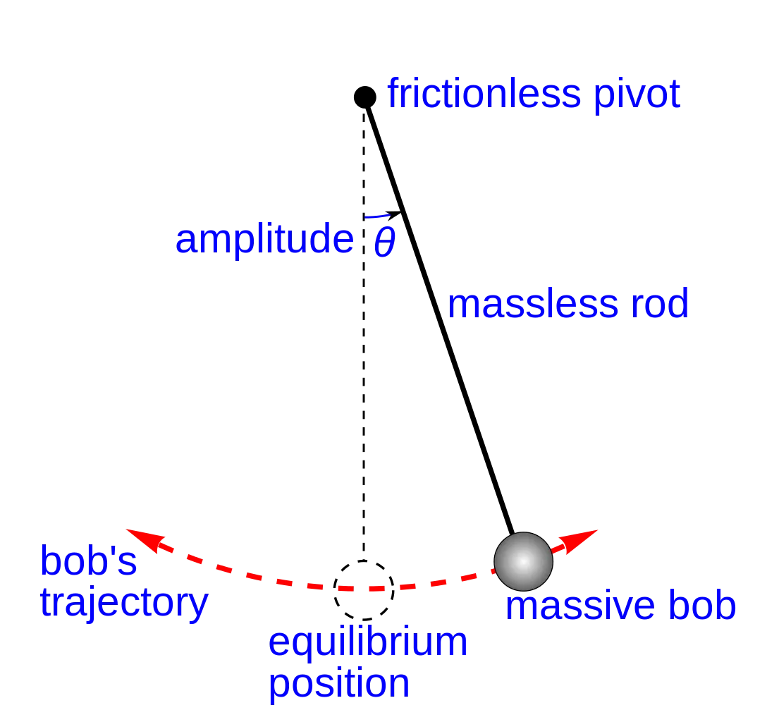
It is said that Galileo measured the periods of a swinging chandelier in church by his pulse beats. He observed that the motion of the chandelier was periodic. The system is a kind of pendulum. This periodic motion is simple harmonic for small displacements from mean position.

Simple Harmonic Motion:

Simple harmonic motion is a special type of periodic motion where displacement is sinusoidal function of time. In SHM, the restoring force on the moving object is directly proportional to and opposite of the object's displacement vector. It results in an oscillation which in absence of drag or any other dissipation of energy, continues indefinitely.

Damped Simple Harmonic Motion:

We know that the motion of a simple pendulum swinging in air, dies out eventually. This happens because the air drag and the friction at the support oppose the motion of the pendulum and dissipate its energy gradually. The pendulum is said to execute damped oscillations. In damped oscillations the energy of the system is dissipated continuously, but for small damping the oscillations remain approximately periodic.

Ordinary Differntial Equations:

An ordinary differential equation (ODE) are derivatives which contain one or more dependant variables and an independant variable. The term ordinary is used in contrast with partial differentials (PDEs can have more than one independant variables). An ODE can be calssified as linear, non-linear, homogenous and non-homogenous. Based on the order of equation, we have, first order, second order, 'nth' order (where n is a natural number) equation. In engineering, ODE is used to descibe the transient behaviour of a system and our interest for this project lies in pendulum.

Dynamics of Pendulum:

For predicting the motion of pedulum, we need to understand the dynamics and the equation that governs its motion. In general, motion of a pendulum can be considered simple harmonic and hence is given by:

`(d^2theta)/(dt^2)+(g/l)sintheta = 0`

where,

• `theta` = angular displacemnt of pendulum bob
• `t` = time (in sec)
• `g` = acceleration due to gravity
• `l` = length of string

But in actual practice motion of pendulum is damped due to dissipative effects. Hence, we need to introduce correction terms:

`(d^2theta)/(dt^2) + b/m((d theta)/dt) +(g/l)sintheta = 0`

where,

`b` = damping coefficient

`m` = mass of pendulum bob (in kg)

This is differential equation of second order and we will use this to simulate the pendulum. But we need to simplify it. We'll use matrix method to do so.

Solution of ODE by matrix method:

Let `theta` be the angular displacement, then angular velocity will be,

`theta = theta1`

`(d theta)/(dt) = theta2`

`(d^2theta)/(dt^2) = d/dt((d theta)/dt) = (d theta2)/(dt)`

Substituting the above in damped ODE for pedulum we get;

`(d theta2)/(dt) + b/m theta2 + g/l sintheta1 = 0`

hence we arrive at these first order ODEs

`:. (d theta1)/(dt) = theta2`

`:. (d theta2)/(dt) = - (b/m theta2 + g/l sintheta1)`

Which can be written in matrix form as,

`d/dt [[theta1], [theta2]] = [[theta2],[- (b/m theta2 + g/l sintheta1)]]`

where,

• `theta1` = Angular displacement of pendulum bob
• `theta2` = Angular velocity of pendulum bob

Program:

The above equation when blended with logic of programming gives following result. The program is written in MATLAB programming language.

But first we need to define a function where we will call our inputs to solve the DE

function [dtheta_dt] = pendulum_characteristics(t,theta,b,g,l,m)
%function to form matrix of the DE
theta1 = theta(1);
theta2 = theta(2);
dtheta1_dt = theta2;
dtheta2_dt = -(b/m)*theta2 - (g/l)*sin(theta1);
dtheta_dt = [dtheta1_dt; dtheta2_dt];
end

This function code is based on the matrix which we derived. Here the first value of LHS row matrix is defined as 'theta1' and second value is defined as 'theta2'. Then all the corresponding equations and relations are entered. This function which is named as 'pendulum_characteristics' is then called in a prebuilt solver called ode45.

The main code is

%Solving Second Order ODE
clear all
close all
clc

%Inputs
b = 0.05;     %damping coefficient
g = 9.81;     %acceleration due to gravity in m/s2
l = 1;        %length of the pendulum in m
m = 1;        %mass of the pendulum bob in kg

%Initial condition
theta_0 = [0;3];

%Time span
t_span = linspace(0,20,500);

%Solving ODE
[t,y] = ode45(@(t,theta) pendulum_characteristics(t,theta,b,g,l,m),t_span,theta_0);

%Plotting Angular displacement and Angular velocity w.r.t Time
colour = [rand rand rand];
hold on
grid on
plot(t,y(:,1),'linewidth',2,'color',colour)
colour = [rand*0.5 rand*0.4 rand*0.3];
plot(t,y(:,2),'linewidth',2,'color',colour)
axis([0 20 -4 4]);
xlabel('Time (sec)');
ylabel('Angular displacement and Angular velocity')
grid on
title('Damping Effect in Simple Pendulum')
legend('Angular displacement','Angular velocity')
%Text = sprintf("Graph.png");  %FOR OCTAVE
%saveas(1,Text);               %for octave


ct = 1;
for i = 1:length(t_span);    
    x0 = 0;
    y0 = 0;
      
    x1 = l*sin(y(i,1));
    y1 = -l*cos(y(i,1));
    
    %Simulation of motion of Pendulum
    grid on
    plot([x0 x1],[y0 y1],[-0.5 0.5],[0 0],'linewidth',3,'color','k')
    hold on
    plot(x1,y1,'marker','o','markerSize',25,'markerFacecolor','r')
    axis([-1.5 1.5 -1.5 0.5])
    title('Motion of a Simple Pendulum with Damping')
    pause(0.00000000001)
    
    %M(ct) = getframe(gcf);  %FOR MATLAB
    
    %Text = sprintf("Pendulum%d.png",ct);    %FOR OCTAVE
    %saveas(1,Text);
    
    ct=ct+1;
    hold off
end

% THE FOLLOWING CODE WORKS FOR MATLAB
%Animation of motion of Simple Pendulum
%movie(M)
%videofile = VideoWriter('Simple_Pendulum.avi','Uncompressed AVI')
%open(videofile)
%writeVideo(videofile,M)
%close(videofile)

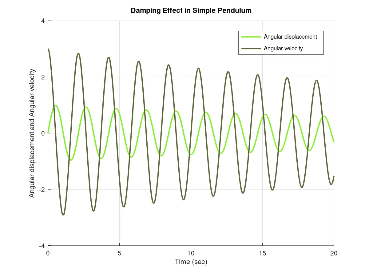
In this code, we gave `b`,`g`,`l` as inputs. Time span was taken as 20 with 500 equal intervals. All this was fed to the function we created (pendulum_characteristics) to solve our DE. The results were stored in [t,y]. Plotting this gave us the follwing results; y(1) and t gave us angular displacement as a function of time and y(2) and t gave us angular velocity as a function of time. Then we initiated a for loop having iterations equal to the length of t_span. In this for loop we plotted the various positions of pendulum bob and sing a loop counter ct we saved each plot as an image file. Later this images were stitched together to form an animation.

Outputs:

Result and Conclusion:

• The angular displacement and angular velocity are sinusoidal for for a pendulum. As the motion is damped, the amplitude of motion reduces gradually.
• The time taken for pendulum to stop is inversely proportional to the damping coefficient. Higher the damping coefficient, earlier the pendulum seizes its motion and vice versa.

References:

• MATLAB for Mechanical Engineers - Course provided by Skill Lync
• GNU Octave
• Supporting Material: Physics - II, Textbook for Class XI - NCERT
• Supporting Material: Higher Engineering Mathematics - BS Grewal
• Supporting Material: Wikimedia

Material: Code and other files