Week 3 - Adiabatic Flame Temperature calculation
1. Adiabatic flame temperature variation with Equivalence ratio (In constant volume-chamber)
We know that
`H = U + PV`
So `U = H - PV`
But `PV = nRT`
So for one mole of an ideal gas `u = h - RT`
The above concept has been used to calculate the internal energy in the following code as the system has been assumed to be under constant volume and not constant pressure.
Moreover, the lean and rich mixtures have different reactions as given below:
For `phi <= 1`(Lean or Stoichiometric mixture)
`phi*CH4 + 2(O2 + 3.76N2) ==> phi*CO2 + phi*2*H20 + 7.52N2 + (1-phi)*2*O2`
For `phi > 1`
`phi*CH4 + 2(O2 + 3.76N2) ==> (4-3*phi) CO2 + 2*phi*H20 + 7.52N2 + 4*(phi - 1)*CO`
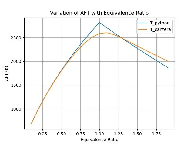
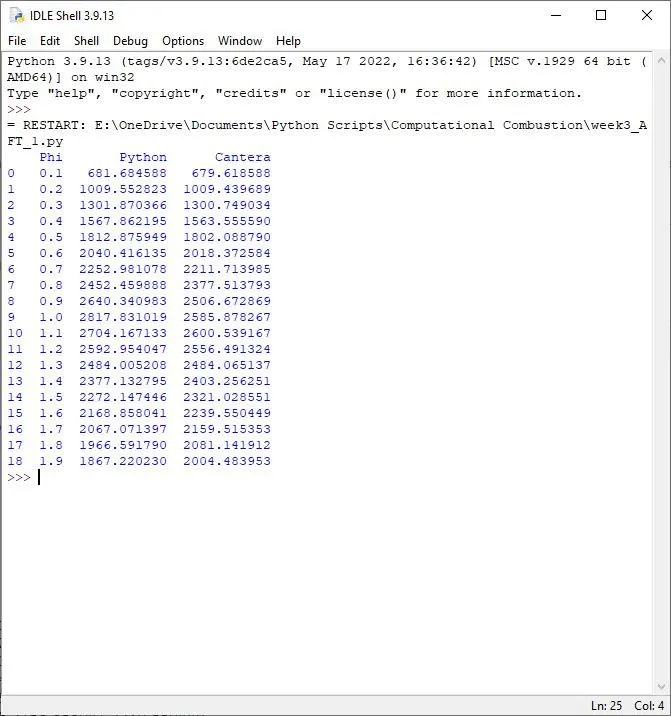
The code for the calculation of AFT with variation in the equivalence ratio using both python and Cantera is attached below:
'''
Adiabatic flame temperature variation with Equivalence ratio (In constant-volume chamber).

For lean (phi<1) and stoichiometric mixtures (phi = 1):
phi*CH4 + 2(O2 + 3.76N2) ==> phi*CO2 + phi*2*H20 + 7.52N2 + (1-phi)*2*O2

For rich mixtures (phi>1):
phi*CH4 + 2(O2 + 3.76N2) ==> (4-3*phi) CO2 + 2*phi*H20 + 7.52N2 + 4*(phi - 1)*CO
'''

import cantera as ct
import numpy as np
import matplotlib.pyplot as plt
import math

#Equivalence ratio range
phi = np.arange(0.1,2,0.1)


#Coefficients for the NASA polynomial to calculate internal energy

ch4_coeffs_l = [5.14987613E+00, -1.36709788E-02, 4.91800599E-05, -4.84743026E-08, 1.66693956E-11, -1.02466476E+04, -4.64130376E+00]

ch4_coeffs_h = [7.48514950E-02, 1.33909467E-02, -5.73285809E-06, 1.22292535E-09, -1.01815230E-13, -9.46834459E+03, 1.84373180E+01]

o2_coeffs_l = [3.78245636E+00, -2.99673416E-03, 9.84730201E-06, -9.68129509E-09, 3.24372837E-12, -1.06394356E+03, 3.65767573E+00]

o2_coeffs_h = [3.28253784E+00, 1.48308754E-03, -7.57966669E-07, 2.09470555E-10, -2.16717794E-14, -1.08845772E+03, 5.45323129E+00]

n2_coeffs_l = [0.03298677E+02, 0.14082404E-02, -0.03963222E-04, 0.05641515E-07, -0.02444854E-10, -0.10208999E+04, 0.03950372E+02]

n2_coeffs_h = [0.02926640E+02, 0.14879768E-02, -0.05684760E-05, 0.10097038E-09, -0.06753351E-13, -0.09227977E+04, 0.05980528E+02]

co2_coeffs_h = [3.85746029E+00, 4.41437026E-03, -2.21481404E-06, 5.23490188E-10, -4.72084164E-14, -4.87591660E+04, 2.27163806E+00]

h20_coeffs_h = [3.03399249E+00, 2.17691804E-03, -1.64072518E-07, -9.70419870E-11, 1.68200992E-14, -3.00042971E+04, 4.96677010E+00]

co_coeffs_h = [2.71518561E+00, 2.06252743E-03,-9.98825771E-07, 2.30053008E-10, -2.03647716E-14, -1.41518724E+04, 7.81868772E+00]


#Function to calculate internal energy
def u(T,coeffs):

    R = 8.314 #J/mol-K
    a1 = coeffs[0]
    a2 = coeffs[1]
    a3 = coeffs[2]
    a4 = coeffs[3]
    a5 = coeffs[4]
    a6 = coeffs[5]

    return (a1 + a2*T/2 + a3*pow(T,2)/3 + a4*pow(T,3)/4 + a5*pow(T,4)/5 + a6/T)*R*T - R*T


def f_u(T, ph):

    #Function that represents the root finding problem

    u_co2_p = u(T, co2_coeffs_h)
    u_h20_p = u(T, h20_coeffs_h)
    u_n2_p = u(T, n2_coeffs_h)
    u_o2_p = u(T, o2_coeffs_h)
    u_co_p = u(T, co_coeffs_h)

    Tstd = 298.15
    u_ch4_r = u(Tstd, ch4_coeffs_l)
    u_o2_r = u(Tstd, o2_coeffs_l)
    u_n2_r = u(Tstd, n2_coeffs_l)

    if ph <= 1:
        u_products = ph*u_co2_p + ph*2*u_h20_p + 7.52*u_n2_p + (1-ph)*2*u_o2_p
        u_reactants = ph*u_ch4_r + 2*u_o2_r + 7.52*u_n2_r
    else:
        u_products = (4-3*ph)*u_co2_p + 2*ph*u_h20_p + 7.52*u_n2_p + 4*(ph-1)*u_co_p
        u_reactants = ph*u_ch4_r + 2*u_o2_r + 7.52*u_n2_r

    return (u_products - u_reactants)

def fprime_u(T,ph):

    return ((f_u(T+1e-6, ph) - f_u(T, ph))/1e-6)

T_guess = 1500
tol = 1e-3
ct_ = 0
alpha = 0.2
T_guess_u = T_guess
ct_u = ct_

T_cv_python = []

for ph in phi:

    while(abs(f_u(T_guess_u,ph)) > tol):

        T_guess_u = T_guess_u - alpha*(f_u(T_guess_u,ph)/fprime_u(T_guess_u,ph))
        ct_u = ct_u + 1

    T_cv_python.append(T_guess_u)

plt.plot(phi,T_cv_python,label = 'T_python')

#==========================Calculation using Cantera===============================

T_cv_cantera = []
gas = ct.Solution('gri30.yaml')

for i in range(len(phi)):

    gas.TPX = 298.15, ct.one_atm, {'CH4':phi[i], 'O2':2, 'N2':7.52}
    gas.equilibrate('UV','auto')
    T_cv_cantera.append(gas.T)

plt.plot(phi, T_cv_cantera, label = 'T_cantera')
plt.xlabel('Equivalence Ratio')
plt.ylabel('AFT (K)')
plt.title('Variation of AFT with Equivalence Ratio')
plt.grid()
plt.legend()
plt.show()

import pandas as pd
df = pd.DataFrame()
df['Phi'] = phi
df['Python'] = T_cv_python
df['Cantera'] = T_cv_cantera
print(df)
PLOT:
OUTPUT SCREEN:
2. Flame temperature variation with Heat loss (In constant pressure-chamber) :
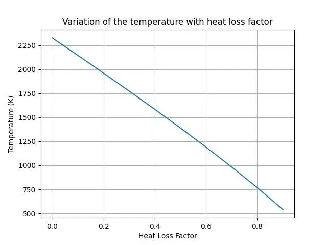
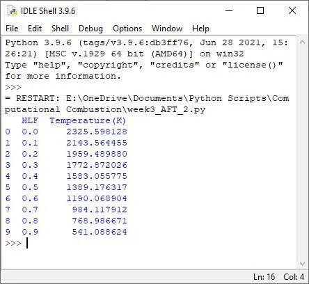
The solution is the same as calculating the AFT at constant pressure conditions except the fact that we need to also consider heat being lost while calculating the change in enthalpy of the gas mixture. This was done as given in the following equation:
`(h_p - h_r) + hlf*Q_(loss)`
Where `hlf`=Heat Loss Factor as fraction of heat lost and `Q_(loss)`= Maximum Possible Heat loss computed as per the formula given
CODE:
'''
Q. Flame temperature variation with Heat loss (In constant pressure-chamber) :

Consider a constant pressure reactor with heat loss.
The reactor is initially set at STP conditions.
The maximum heat loss for the reaction is given below.
You will vary the heat loss term by multiplying the
“maximum heat loss” with a factor known as H_loss_factor.
Example, H_loss_factor = 0.5 would mean a heat loss for that
reaction that is equal to 50% of the maximum possible heat loss.
'''

import cantera as ct
import numpy as np
import matplotlib.pyplot as plt
import math

#Equivalence ratio range

#Equivalence Ratio
ph = 1

#Heat loss factor
hl = np.arange(0,1,0.1)


#Coefficients for the NASA polynomial to calculate enthalpy and internal energy

ch4_coeffs_l = [5.14987613E+00, -1.36709788E-02, 4.91800599E-05, -4.84743026E-08, 1.66693956E-11, -1.02466476E+04, -4.64130376E+00]

ch4_coeffs_h = [7.48514950E-02, 1.33909467E-02, -5.73285809E-06, 1.22292535E-09, -1.01815230E-13, -9.46834459E+03, 1.84373180E+01]

o2_coeffs_l = [3.78245636E+00, -2.99673416E-03, 9.84730201E-06, -9.68129509E-09, 3.24372837E-12, -1.06394356E+03, 3.65767573E+00]

o2_coeffs_h = [3.28253784E+00, 1.48308754E-03, -7.57966669E-07, 2.09470555E-10, -2.16717794E-14, -1.08845772E+03, 5.45323129E+00]

n2_coeffs_l = [0.03298677E+02, 0.14082404E-02, -0.03963222E-04, 0.05641515E-07, -0.02444854E-10, -0.10208999E+04, 0.03950372E+02]

n2_coeffs_h = [0.02926640E+02, 0.14879768E-02, -0.05684760E-05, 0.10097038E-09, -0.06753351E-13, -0.09227977E+04, 0.05980528E+02]

co2_coeffs_l = [2.35677352E+00, 8.98459677E-03, -7.12356269E-06, 2.45919022E-09, -1.43699548E-13, -4.83719697E+04, 9.90105222E+00]

co2_coeffs_h = [3.85746029E+00, 4.41437026E-03, -2.21481404E-06, 5.23490188E-10, -4.72084164E-14, -4.87591660E+04, 2.27163806E+00]

h20_coeffs_l = [4.19864056E+00,-2.03643410E-03, 6.52040211E-06, -5.48797062E-09, 1.77197817E-12, -3.02937267E+04, -8.49032208E-01]

h20_coeffs_h = [3.03399249E+00, 2.17691804E-03, -1.64072518E-07, -9.70419870E-11, 1.68200992E-14, -3.00042971E+04, 4.96677010E+00]

co_coeffs_l = [3.57953347E+00,-6.10353680E-04, 1.01681433E-06, 9.07005884E-10, -9.04424499E-13, -1.43440860E+04, 3.50840928E+00]

co_coeffs_h = [2.71518561E+00, 2.06252743E-03,-9.98825771E-07, 2.30053008E-10, -2.03647716E-14, -1.41518724E+04, 7.81868772E+00]

#Function to calculate enthalpy
def h(T,coeffs):

    R = 8.314 #J/mol-K
    a1 = coeffs[0]
    a2 = coeffs[1]
    a3 = coeffs[2]
    a4 = coeffs[3]
    a5 = coeffs[4]
    a6 = coeffs[5]

    return (a1 + a2*T/2 + a3*pow(T,2)/3 + a4*pow(T,3)/4 + a5*pow(T,4)/5 + a6/T)*R*T


def f_h(T, ph, hlf):

    #Function that represents the root finding problem

    h_co2_p = h(T, co2_coeffs_h)
    h_h20_p = h(T, h20_coeffs_h)
    h_n2_p = h(T, n2_coeffs_h)
    h_o2_p = h(T, o2_coeffs_h)
    h_co_p = h(T, co_coeffs_h)

    Tstd = 298.15
    h_ch4_r = h(Tstd, ch4_coeffs_l)
    h_o2_r = h(Tstd, o2_coeffs_l)
    h_n2_r = h(Tstd, n2_coeffs_l)

    Q_hl_max = 0
    h_co2_p_max = h(Tstd , co2_coeffs_l)
    h_h20_p_max = h(Tstd , h20_coeffs_l)
    h_n2_p_max = h(Tstd , n2_coeffs_l)
    h_o2_p_max = h(Tstd , o2_coeffs_l)
    h_co_p_max = h(Tstd , co_coeffs_l)


    if ph <= 1:
        h_products = ph*h_co2_p + ph*2*h_h20_p + 7.52*h_n2_p + (1-ph)*2*h_o2_p
        h_reactants = ph*h_ch4_r + 2*h_o2_r+ 7.52*h_n2_r
        h_products_max = ph*h_co2_p_max + ph*2*h_h20_p_max+ 7.52*h_n2_p_max + (1-ph)*2*h_o2_p_max
        Q_hl_max = h_reactants - h_products_max  #Maximum possible Heat Loss

    else:
        h_products = (4-3*ph)*h_co2_p + 2*ph*h_h20_p + 7.52*h_n2_p + 4*(ph-1)*h_co_p
        h_reactants = ph*h_ch4_r + 2*h_o2_r+ 7.52*h_n2_r
        h_products_max = (4-3*ph)*h_co2_p_max + 2*ph*h_h20_p_max + 7.52*h_n2_p_max + 4*(ph-1)*h_co_p_max
        Q_hl_max = h_reactants - h_products_max  #Maximum possible Heat Loss

    return (h_products - h_reactants) + hlf*Q_hl_max


def fprime_h(T,ph,hlf):

    return ((f_h(T+1e-6, ph, hlf) - f_h(T, ph, hlf))/1e-6)

#Initial conditions for Newton_Raphson method
T_guess = 1000
tol = 1e-3
ct_ = 0
alpha = 0.2
T_guess_h = T_guess
ct_h = ct_

T_cp_python = []

#Implementing Newton-Raphson for all the values of heat loss factor
for hlf in hl:

    while(abs(f_h(T_guess_h,ph,hlf)) > tol):

        T_guess_h = T_guess_h - alpha*(f_h(T_guess_h,ph,hlf)/fprime_h(T_guess_h,ph,hlf))
        ct_h = ct_h + 1

    T_cp_python.append(T_guess_h)

#Plotting the results
plt.plot(hl,T_cp_python)
plt.xlabel('Heat Loss Factor')
plt.ylabel('Temperature (K)')
plt.title('Variation of the temperature with heat loss factor')
plt.grid()

#Displaying the results in a data frame
import pandas as pd
df = pd.DataFrame(columns = ['HLF','Temperature(K)'])
df['HLF'] = hl
df['Temperature(K)'] = T_cp_python
print(df)

plt.show()
PLOT:
OUTPUT SCREEN:
3. Adiabatic flame temperature variation with respect to Alkane, Alkene, Alkyne :
Alkane: Carbon compound where the carbon atoms have only single bond between them and are called as saturated hydrocarbons. They are represented by a general formula of `C_nH_(2n+2)`. Example - Methane `(CH_4)`.
Alkene: Carbon compound where at least one carbon-carbon bond is a double bond. They are represented by a general formula `C_nH_(2n)`. Example- Ethene `(C_2H_4)`.
Alkyne: Carbon compound where atleat one carbon-carbon triple bond exists. It has a general formula `C_nH_(2n-2)`. Example - Ethyne `(C_2H_2)`.
Alkene and alkyne are also called as unsaturated hydrocarbons.
The general equation for combustion for a hydrocarbon is of the following form:
`C_xH_y + (x + y/4)O_2 -> xCO_2 + y/2H_2O`
CODE:
'''
3. Adiabatic flame temperature variation with respect to Alkane, Alkene, Alkyne :

Test it only for Alk -ane, -ene and -yne variants of 2 Carbon atom
chains and plot a trend Assume no heat loss.
Note: Use python coding logic as cantera requires reaction
mechanism file and ‘gri30.xml’ file is specifically for methane as fuel.
'''

import cantera as ct
import numpy as np
import matplotlib.pyplot as plt
import math

#Coefficients for the NASA polynomial to calculate enthalpy and internal energy

##ALKYNE
c2h2_coeffs_l = [8.08681094E-01, 2.33615629E-02, -3.55171815E-05, 2.80152437E-08, -8.50072974E-12, 2.64289807E+04, 1.39397051E+01]

c2h2_coeffs_h = [4.14756964E+00, 5.96166664E-03, -2.37294852E-06, 4.67412171E-10, -3.61235213E-14, 2.59359992E+04, -1.23028121E+00]

##ALKENE
c2h4_coeffs_l = [3.95920148E+00, -7.57052247E-03, 5.70990292E-05, -6.91588753E-08, 2.69884373E-11, 5.08977593E+03, 4.09733096E+00]

c2h4_coeffs_h = [2.03611116E+00, 1.46454151E-02, -6.71077915E-06, 1.47222923E-09, -1.25706061E-13, 4.93988614E+03, 1.03053693E+01]

##ALKANE
c2h6_coeffs_l = [4.29142492E+00, -5.50154270E-03, 5.99438288E-05, -7.08466285E-08, 2.68685771E-11, -1.15222055E+04, 2.66682316E+00]

c2h6_coeffs_h = [1.07188150E+00, 2.16852677E-02, -1.00256067E-05, 2.21412001E-09, -1.90002890E-13, -1.14263932E+04, 1.51156107E+01]

#Dictionary storing the no of carbon and hydrogen atoms and the respective coefficients for calculation of the enthalpies
gas = dict()
gas['alkane'] = [2,6,c2h6_coeffs_l, c2h6_coeffs_h]
gas['alkene'] = [2,4,c2h4_coeffs_l, c2h4_coeffs_h]
gas['alkyne'] = [2,2,c2h2_coeffs_l, c2h2_coeffs_h]

o2_coeffs_l = [3.78245636E+00, -2.99673416E-03, 9.84730201E-06, -9.68129509E-09, 3.24372837E-12, -1.06394356E+03, 3.65767573E+00]

o2_coeffs_h = [3.28253784E+00, 1.48308754E-03, -7.57966669E-07, 2.09470555E-10, -2.16717794E-14, -1.08845772E+03, 5.45323129E+00]

n2_coeffs_l = [0.03298677E+02, 0.14082404E-02, -0.03963222E-04, 0.05641515E-07, -0.02444854E-10, -0.10208999E+04, 0.03950372E+02]

n2_coeffs_h = [0.02926640E+02, 0.14879768E-02, -0.05684760E-05, 0.10097038E-09, -0.06753351E-13, -0.09227977E+04, 0.05980528E+02]

co2_coeffs_l = [2.35677352E+00, 8.98459677E-03, -7.12356269E-06, 2.45919022E-09, -1.43699548E-13, -4.83719697E+04, 9.90105222E+00]

co2_coeffs_h = [3.85746029E+00, 4.41437026E-03, -2.21481404E-06, 5.23490188E-10, -4.72084164E-14, -4.87591660E+04, 2.27163806E+00]

h20_coeffs_l = [4.19864056E+00,-2.03643410E-03, 6.52040211E-06, -5.48797062E-09, 1.77197817E-12, -3.02937267E+04, -8.49032208E-01]

h20_coeffs_h = [3.03399249E+00, 2.17691804E-03, -1.64072518E-07, -9.70419870E-11, 1.68200992E-14, -3.00042971E+04, 4.96677010E+00]

co_coeffs_l = [3.57953347E+00,-6.10353680E-04, 1.01681433E-06, 9.07005884E-10, -9.04424499E-13, -1.43440860E+04, 3.50840928E+00]

co_coeffs_h = [2.71518561E+00, 2.06252743E-03,-9.98825771E-07, 2.30053008E-10, -2.03647716E-14, -1.41518724E+04, 7.81868772E+00]

#Function to calculate enthalpy
def h(T,coeffs):

    R = 8.314 #J/mol-K
    a1 = coeffs[0]
    a2 = coeffs[1]
    a3 = coeffs[2]
    a4 = coeffs[3]
    a5 = coeffs[4]
    a6 = coeffs[5]

    return (a1 + a2*T/2 + a3*pow(T,2)/3 + a4*pow(T,3)/4 + a5*pow(T,4)/5 + a6/T)*R*T

def f_h(T, k):

    #Function that represents the root finding problem

    h_co2_p = h(T, co2_coeffs_h)
    h_h20_p = h(T, h20_coeffs_h)
    h_n2_p = h(T, n2_coeffs_h)
    h_o2_p = h(T, o2_coeffs_h)
    h_co_p = h(T, co_coeffs_h)

    Tstd = 298.15
    h_gas_r = h(Tstd, gas[k][2])
    h_o2_r = h(Tstd, o2_coeffs_l)
    h_n2_r = h(Tstd, n2_coeffs_l)

    x = gas[k][0]
    y = gas[k][1]
    a = x + y/4;
    h_products = x*h_co2_p + (y/2)*h_h20_p + 3.76*a*h_n2_p
    h_reactants = h_gas_r + a*h_o2_r+ 3.76*a*h_n2_r

    return (h_products - h_reactants)


def fprime_h(T,k):

    return ((f_h(T+1e-6,k) - f_h(T,k))/1e-6)

#Intial conditions for Newton-Raphson Method
T_guess = 1000
tol = 1e-3
ct_ = 0
alpha = 0.2
T_guess_h = T_guess
ct_h = ct_

T_cp_python = []

#Loop to calculate AFT for alkane, alkene and alkyne using Newton-Raphson method
for k in list(gas.keys()):

    while(abs(f_h(T_guess_h,k)) > tol):

        T_guess_h = T_guess_h - alpha*(f_h(T_guess_h,k)/fprime_h(T_guess_h,k))
        ct_h = ct_h + 1

    T_cp_python.append(T_guess_h)

print('AFT for Alkane(C2H6):',T_cp_python[0])
print('AFT for Alkene(C2H4):',T_cp_python[1])
print('AFT for Alkyne(C2H2):',T_cp_python[2])

plt.plot(list(gas.keys()),T_cp_python,label = 'T_python_cp')
plt.xlabel('Hydrocarbon Type')
plt.ylabel('AFT (K)')
plt.grid()
plt.title('Variation of AFT with Alkane, Alekene and Alkyne')
plt.show()
PLOT:
OUTPUT SCREEN:
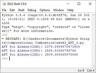
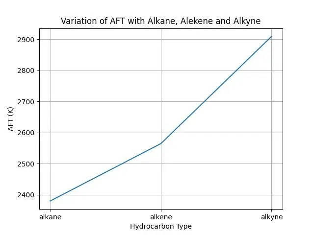
As expected the AFT is higher for compounds having double and triple bond as higher energy is released when a triple bond is broken as compared to a double or a single bond between the carbon atoms.
4. Adiabatic flame temperature variation with respect to number of Carbon atom chains :
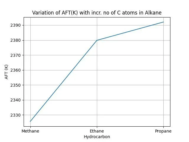
Here again we consider 3 alkanes with increasing number of carbon atoms, namely, Methane, Ethane and Propane and observe their AFTs. The general equation for combustion stays the same as mentioned in the above answer.
CODE:
'''
4. Adiabatic flame temperature variation with respect to number of Carbon atom chains :

For a general alkane, plot the effect of the number of carbon atoms (from 1 to 3)
on the final temperature. Assume no heat loss.

Note: Use python coding logic as cantera requires reaction mechanism file and
‘gri30.xml’ file is specifically for methane as fuel.
'''

import cantera as ct
import numpy as np
import matplotlib.pyplot as plt
import math

#Coefficients for the NASA polynomial to calculate enthalpy and internal energy

##METHANE
ch4_coeffs_l = [5.14987613E+00, -1.36709788E-02, 4.91800599E-05, -4.84743026E-08, 1.66693956E-11, -1.02466476E+04, -4.64130376E+00]

ch4_coeffs_h = [7.48514950E-02, 1.33909467E-02, -5.73285809E-06, 1.22292535E-09, -1.01815230E-13, -9.46834459E+03, 1.84373180E+01]

##ETHANE
c2h6_coeffs_l = [4.29142492E+00, -5.50154270E-03, 5.99438288E-05, -7.08466285E-08, 2.68685771E-11, -1.15222055E+04, 2.66682316E+00]

c2h6_coeffs_h = [1.07188150E+00, 2.16852677E-02, -1.00256067E-05, 2.21412001E-09, -1.90002890E-13, -1.14263932E+04, 1.51156107E+01]

##PROPANE
c3h8_coeffs_l = [0.93355381E+00, 0.26424579E-01, 0.61059727E-05, -0.21977499E-07, 0.95149253E-11, -0.13958520E+05, 0.19201691E+02]

c3h8_coeffs_h = [0.75341368E+01, 0.18872239E-01, -0.62718491E-05, 0.91475649E-09, -0.47838069E-13, -0.16467516E+05, -0.17892349E+02]


gas = dict() #Dictionary to store no of carbon and hydrogen atoms and the coefficients for enthalpy calculation

gas['Methane'] = [1,4, ch4_coeffs_l, ch4_coeffs_h]

gas['Ethane'] = [2,6, c2h6_coeffs_l, c2h6_coeffs_h]

gas['Propane'] = [3,8, c3h8_coeffs_l, c3h8_coeffs_h]

o2_coeffs_l = [3.78245636E+00, -2.99673416E-03, 9.84730201E-06, -9.68129509E-09, 3.24372837E-12, -1.06394356E+03, 3.65767573E+00]

o2_coeffs_h = [3.28253784E+00, 1.48308754E-03, -7.57966669E-07, 2.09470555E-10, -2.16717794E-14, -1.08845772E+03, 5.45323129E+00]

n2_coeffs_l = [0.03298677E+02, 0.14082404E-02, -0.03963222E-04, 0.05641515E-07, -0.02444854E-10, -0.10208999E+04, 0.03950372E+02]

n2_coeffs_h = [0.02926640E+02, 0.14879768E-02, -0.05684760E-05, 0.10097038E-09, -0.06753351E-13, -0.09227977E+04, 0.05980528E+02]

co2_coeffs_l = [2.35677352E+00, 8.98459677E-03, -7.12356269E-06, 2.45919022E-09, -1.43699548E-13, -4.83719697E+04, 9.90105222E+00]

co2_coeffs_h = [3.85746029E+00, 4.41437026E-03, -2.21481404E-06, 5.23490188E-10, -4.72084164E-14, -4.87591660E+04, 2.27163806E+00]

h20_coeffs_l = [4.19864056E+00,-2.03643410E-03, 6.52040211E-06, -5.48797062E-09, 1.77197817E-12, -3.02937267E+04, -8.49032208E-01]

h20_coeffs_h = [3.03399249E+00, 2.17691804E-03, -1.64072518E-07, -9.70419870E-11, 1.68200992E-14, -3.00042971E+04, 4.96677010E+00]

#Function to calculate enthalpy
def h(T,coeffs):

    R = 8.314 #J/mol-K
    a1 = coeffs[0]
    a2 = coeffs[1]
    a3 = coeffs[2]
    a4 = coeffs[3]
    a5 = coeffs[4]
    a6 = coeffs[5]

    return (a1 + a2*T/2 + a3*pow(T,2)/3 + a4*pow(T,3)/4 + a5*pow(T,4)/5 + a6/T)*R*T

def f_h(T, k):

    #Function that represents the root finding problem

    h_co2_p = h(T, co2_coeffs_h)
    h_h20_p = h(T, h20_coeffs_h)
    h_n2_p = h(T, n2_coeffs_h)

    Tstd = 298.15
    h_gas_r = h(Tstd, gas[k][2])
    h_o2_r = h(Tstd, o2_coeffs_l)
    h_n2_r = h(Tstd, n2_coeffs_l)

    x = gas[k][0] #No of carbon atoms
    y = gas[k][1] #No of hydrogen atoms
    a = x + y/4;
    h_products = x*h_co2_p + (y/2)*h_h20_p + 3.76*a*h_n2_p
    h_reactants = h_gas_r + a*h_o2_r+ 3.76*a*h_n2_r

    return (h_products - h_reactants)


def fprime_h(T,k):

    return ((f_h(T+1e-6,k) - f_h(T,k))/1e-6)


T_guess = 1000
tol = 1e-3
ct_ = 0
alpha = 0.2
T_guess_h = T_guess
ct_h = ct_

T_cp_python = []


for k in list(gas.keys()):

    while(abs(f_h(T_guess_h,k)) > tol):

        T_guess_h = T_guess_h - alpha*(f_h(T_guess_h,k)/fprime_h(T_guess_h,k))
        #plt.plot(ct_h,T_guess_h,'*',color = 'red')
        ct_h = ct_h + 1

    T_cp_python.append(T_guess_h)


#print('Temperature = ', T_guess_h)

print('AFT for Methane:',T_cp_python[0])
print('AFT for Ethane:',T_cp_python[1])
print('AFT for Propane:',T_cp_python[2])
plt.plot(list(gas.keys()),T_cp_python,label = 'T_python_cp')
plt.xlabel('Hydrocarbon')
plt.ylabel('AFT (K)')
plt.grid()
plt.title('Variation of AFT(K) with incr. no of C atoms in Alkane')
plt.show()
PLOT:
OUTPUT SCREEN:
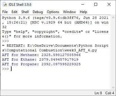
It could be observed that the AFT increases with increasing no of carbon atoms as larger no of bonds broken release greater amount of energy. This completes the answer of all the four questions.