Week 3.5 - Deriving 4th order approximation of a 2nd order derivative using Taylor Table method

Objective: Derive the following 4th order approximations of the second-order derivative.

1. Central difference

2. Skewed right-sided difference

3. Skewed left-sided difference

After deriving these schemes, prove that your skewed schemes are fourth-order accurate

Derivation:

1. Central differencing scheme

	f(i)	f'(i)*`trianglex`	f''(i)*`trianglex^2`	f'''(i)*`trianglex^3`	f''''(i)*`trianglex^4`	f'''''(i)*`trianglex^5`
f(i-2)	a	-2a	4a/2!	8a/3!	16a/4!	32a/5!
f(i-1)	b	-b	b/2!	-b/3!	b/4!	-b/5!
f(i)	c	0	0	0	0	0
f(i+1)	d	d	d/2!	d/3!	d/4!	d/5!
f(i+2)	e	2e	4e/2!	8e/3!	16e/4!	32e/5!
	0	0	1	0	0	0

2. Skewed right-sided difference

	f(i)	f'(i)*`trianglex`	f''(i)*`trianglex^2`	f'''(i)*`trianglex^3`	f''''(i)*`trianglex^4`	f'''''(i)*`trianglex^5`
f(i)	a	0	0	0	0	0
f(i+1)	b	b	b/2!	b/3!	b/4!	b/5!
f(i+2)	c	2c	4c/2!	8c/3!	16c/4!	32c/5!
f(i+3)	d	3d	9d/2!	27d/3!	81d/4!	243d/5!
f(i+4)	e	4e	16e/2!	64e/3!	256e/4!	1024e/5!
f(i+5)	f	5f	25f/2!	125f/3!	625f/4!	3125f/5!
	0	0	1	0	0	0

2. Skewed left-sided difference

	f(i)	f'(i)*`trianglex`	f''(i)*`trianglex^2`	f'''(i)*`trianglex^3`	f''''(i)*`trianglex^4`	f'''''(i)*`trianglex^5`
f(i-5)	a	-5a	25a/2!	-125a/3!	625a/4!	-3125a/5!
f(i-4)	b	-4b	16b/2!	-64b/3!	256b/4!	-1024b/5!
f(i-3)	c	-3c	9c/2!	-27c/3!	81c/4!	-243c/5!
f(i-2)	d	-2d	4d/2!	-8d/3!	16d/4!	-32d/5!
f(i-1)	e	-e	e/2!	-e/3!	e/4!	-e/5!
f(i)	f	0	0	0	0	0
	0	0	1	0	0	0

Main Code:

clear all
close all
clc

order_Approx = input('What is the order of approximation :');
order_derv = input('What is the order of derivtive :');
% grid_point = order_Approx+order_derv;
x= pi/3;
dx = linspace(pi/4,pi/400,100);
%analytical
analytical_derv = -2*exp(x)*sin(x);

%Central difference scheme
[out_cd] = c_d(order_Approx,order_derv,x,dx);
error_cd = abs(out_cd-analytical_derv);

%Skewed left
[out_l_s_d] = l_s_d(order_Approx,order_derv,x,dx);
error_l_s_d = abs(out_l_s_d-analytical_derv);

%Skewed Right
[out_r_s_d] = r_s_d(order_Approx,order_derv,x,dx);
error_r_s_d = abs(out_r_s_d-analytical_derv);

loglog(dx,error_cd,'linewidth',2)
hold on
loglog(dx,error_l_s_d,'linewidth',2)
hold on
loglog(dx,error_r_s_d,'linewidth',2)
xlabel('Error');
ylabel('dx');
legend('Central differencing','Skewed left sided','Skewed right-sided','location','northwest');

Function code:

Central differencing scheme

function [out_cd] = c_d(order_Approx,order_derv,x,dx)
c_d_m = 0;

grid_point = order_Approx+order_derv-1;
n = round(-(order_Approx/2));
a = 0;
coeff_matrix = zeros(grid_point);
for row = 1:grid_point
    for coloumn = 1:grid_point
        coeff_matrix(row,coloumn) = ((n)^a/factorial(a));
        a = a+1; 
    end
    n = n+1;
    a = 0;
end
solution = zeros(grid_point,1);
solution(order_derv+1) = 1;
coeff_cd = linsolve(coeff_matrix',solution);
n = round(-(order_Approx/2));
for i = 1:length(coeff_cd)
    c_d_a = (coeff_cd(i)*exp(x+n.*dx).*cos(x+n.*dx)./dx.^order_derv );
    c_d_m = c_d_m+c_d_a;
    n = n+1;
end
out_cd = c_d_m;
end

Skewed right-sided difference

function [out_r_s_d] = r_s_d(order_Approx,order_derv,x,dx)
r_s_d = 0;
grid_point = order_Approx+order_derv;
n = 0;
a = 0;
coeff_matrix = zeros(grid_point);

for row = 1:grid_point
    for coloumn = 1:grid_point
        coeff_matrix(row,coloumn) = ((n)^a/factorial(a));
        a = a+1; 
    end
    n = n+1;
    a = 0;
end

solution = zeros(grid_point,1);
solution(order_derv+1) = 1;
coeff_cd = linsolve(coeff_matrix',solution);
n = 0;
for i = 1:length(coeff_cd)
    c_d_a = (coeff_cd(i)*exp(x+n.*dx).*cos(x+n.*dx)./dx.^order_derv );
    r_s_d = r_s_d+c_d_a;
    n = n+1;
end
out_r_s_d =  r_s_d ;

end

Skewed left-sided difference

function [out_l_s_d] = l_s_d(order_Approx,order_derv,x,dx)

l_s_d = 0;
grid_point = order_Approx+order_derv;
n = -(grid_point-1);
a = 0;
coeff_matrix = zeros(grid_point);

for row = 1:grid_point
    for coloumn = 1:grid_point
        coeff_matrix(row,coloumn) = ((n)^a/factorial(a));
        a = a+1; 
    end
    n = n+1;
    a = 0;
end


solution = zeros(grid_point,1);
solution(order_derv+1) = 1;
coeff_cd = linsolve(coeff_matrix',solution);
n = -(grid_point-1);
for i = 1:length(coeff_cd)
    c_d_a = (coeff_cd(i)*exp(x+n.*dx).*cos(x+n.*dx)./dx.^order_derv );
    l_s_d = l_s_d+c_d_a;
    n = n+1;
end
out_l_s_d = l_s_d;
end

Procedure:

• First, we input the value for the order of approximation and the order of derivative to be found.
• Then initialize the value of x, dx, and compute the analytical derivative value.
• Three functions are defined for the central differencing skewed left-sided scheme and skewed right-sided scheme.
• The difference between the output value and the analytical value is taken for different values of dx.
• The error is plotted with dx.

Results

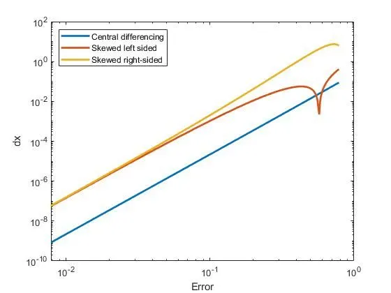
It is clear from the plot that the central differencing scheme gives the least error for the fourth-order approximation of second-order derivative. this can be attributed to the character of central differencing scheme which takes data from both sides whereas the skewed schemes are taking grid points from one side of the point of interest.

The skewed schemes are mainly used in the case of unidirectional flow. That is in the boundary regions,For the central differencing scheme, we would have to introduce grid points outside the domain for the boundary region which would lead to simulation having greater error compared to the skewed schemes.

We can conclude by saying that the central differencing scheme is useful for discretizing the bulk of the domain whereas the skewed (right-sided or left-sided) schemes are useful for mainly unidirectional flow involving boundary condition,