Week 3.5 - Deriving 4th order approximation of a 2nd order derivative using Taylor Table method
AIM: To derive the
4th order approximation of a second order derivative with Central Difference,
Skewed Right Sided Difference and Skewed Left Sided Difference using the
Taylor's Table method.
SOLUTION:
The order of
accuracy of a numerical scheme is given by the following formulae:
P = N - Q + 1
(For Symmetric or Central schemes)
P = N - Q (For
One-Sided or Skewed Schemes)
Where, P =
Order of Accuracy
N =
Number of nodes in the stencil
Q =
Order of derivative
The above
formula clearly shows that if higher order accuracy is desired for a given
order of derivative (Q Constant) then the only way is to increase the the
number of nodes (N) in the stencil being used. However the error also depends
on the step size (del_X) and the type of scheme being used. In this exercise
effect of both of these parameters on the accuracy has been evaluated.
CENTRAL DIFFERENCE SCHEME
For this scheme we get, N = 4 + 2
- 1 = 5 (P = 4 & Q = 2).
Hence we need 5 nodes in our
stencil.
Let us assume the following
approximation for the central difference scheme:
d2u/dx2 = [
a*f(x-2del_x)+b*f(x-del_x)+c*f(x)+d*f(x+del_x)+e*f(x+2del_x) ] / del_x2
Taylors Table:
|
f(x) |
del_x*f'(x) |
del_x2*f2(x) |
del_x3*f3(x) |
del_x4*f4(x) |
|
|
f(x-2del_x) |
a |
-2a |
2a |
-8a/6 |
16a/24 |
|
f(x-del_x) |
b |
-b |
b/2 |
-b/6 |
b/24 |
|
f(x) |
c |
0 |
0 |
0 |
0 |
|
f(x+del_x) |
d |
d |
d/2 |
d/6 |
d/24 |
|
f(x+2del_x) |
e |
2e |
2e |
8e/6 |
16e/24 |
|
SUM |
0 |
0 |
1 |
0 |
0 |
We get the following 5 equations when the entries in each
column is equated to the entry in the sum row in the corresponding column:
a+b+c+d+e = 0
-2a+b+0+d+2e = 0
2a+(b/2)+0+(d/2)+2e = 1
(-8a/6)-(b/6)+0+d/6+8e/6 = 0
16a/24+b/24+0+d/24+16e/24 = 0
The above system of 5 linear equation
with exactly 5 unknowns can be solved by using linsolve(A,B) function in MATLAB
where
A = [ 1 1 1 1 1 ;
-2 -1 0 1 2 ;
4/2 1/2 0 1/2 4/2;
-8/6 -1/6 0 1/6 8/6;
16/24 1/24 0 1/24 16/24];
B = [ 0; 0; 1; 0; 0 ];
This gives us
a = -0.0833, b = 1.3333, c = -2.5000, d = 1.3333, e
= -0.0833
Substituting
the above values the Second order derivative can be obtained for a suitable
value of del_x.
SKEWED RIGHT SIDED DIFFERENCE SCHEME
For this scheme we get, N = 4 +
2 = 6 (P = 4 & Q = 2).
Hence we need 6 nodes in our
stencil.
Let us assume the following
approximation for the skewed right sided difference scheme:
d2u/dx2= [a*f(x)+b*f(x+del_x)+c*f(x+2del_x)+
d*f(x+3del_x) + e*f(x+4del_x)+ g*f(x+5del_x)] /del_x2
Taylors Table:
|
f(x) |
del_x*f1(x) |
del_x2*f2(x) |
del_x3*f3(x) |
del_x4*f4(x) |
del_x5*f5(x) |
|
|
f(x) |
a |
0 |
0 |
0 |
0 |
0 |
|
f(x+del_x) |
b |
b |
b/2 |
b/6 |
b/24 |
b/120 |
|
f(x+2del_x) |
c |
2c |
4c/2 |
8c/6 |
16c/24 |
32c/120 |
|
f(x+3del_x) |
d |
3d |
9d/2 |
27d/6 |
81d/24 |
243d/120 |
|
f(x+4del_x) |
e |
4e |
16e/2 |
64e/6 |
256e/24 |
1024e/120 |
|
f(x+5del_x) |
g |
5g |
25g/2 |
125g/6 |
625g/25 |
3125g/120 |
|
SUM |
0 |
0 |
1 |
0 |
0 |
0 |
We get the following 6 equations when the entries in each
column is equated to the entry in the sum row in the corresponding column:
a+b+c+d+e+g= 0
0+b+2c+3d+4e+5g = 0
0+(b/2)+(4e/2)+(9d/2)+(16e/2)+(25g/2) = 1
0+(b/6)+(8c/6)+(27d/6)+(64e/6)+(125g/6) = 0
0+(b/24)+(16c/24)+(81d/24)+(256e/24)+(625g/24) = 0
0+(b/120)+(32c/120)+(243d/120)+(1024e/120)+(3125g/120) = 0
The above system of 5 linear equation with exactly 5
unknowns can be solved by using linsolve(A,B) function in MATLAB where
A = [ 1 1 1 1 1 1;
0 1 2 3 4 5;
0 1/2 2 9/2 8
25/2;
0 1/6 8/6 27/6
64/6 125/6;
0 1/24 16/24
81/24 256/24 625/24;
0 1/120 32/120
243/120 1024/120 3125/120];
B = [ 0; 0; 1; 0; 0; 0 ];
This gives us a = 3.7500, b = -12.8333, c = 17.8333, d = -13.000,
e = 5.0833 and g = -0.8333
Substituting the above values the Second order derivative can be obtained for a suitable value of del_x.
SKEWED LEFT SIDED DIFFERENCE SCHEME
Again, for this scheme also we
get, N = 4 + 2 = 6 (P = 4 & Q = 2).
Here also we need 6 nodes in our
stencil.
Let us assume the following
approximation for the skewed right sided difference scheme:
d2u/dx2= [a*f(x)+b*f(x-del_x)+c*f(x-2del_x)+
d*f(x-3del_x) + e*f(x-4del_x)+ g*f(x-5del_x)] /del_x2
Taylors Table:
|
f(x) |
del_x*f1(x) |
del_x2*f2(x) |
del_x3*f3(x) |
del_x4*f4(x) |
del_x5*f5(x) |
|
|
f(x) |
a |
0 |
0 |
0 |
0 |
0 |
|
f(x-del_x) |
b |
-b |
b/2 |
-b/6 |
b/24 |
-b/120 |
|
f(x-2del_x) |
c |
-2c |
4c/2 |
-8c/6 |
16c/24 |
-32c/120 |
|
f(x-3del_x) |
d |
-3d |
9d/2 |
-27d/6 |
81d/24 |
-243d/120 |
|
f(x-4del_x) |
e |
-4e |
16e/2 |
-64e/6 |
256e/24 |
-1024e/120 |
|
f(x-5del_x) |
g |
-5g |
25g/2 |
-125g/6 |
625g/25 |
-3125g/120 |
|
SUM |
0 |
0 |
1 |
0 |
0 |
0 |
We get the following 6 equations when the entries in each
column is equated to the entry in the sum row in the corresponding column:
a+b+c+d+e+g= 0
0+b+2c+3d+4e+5g = 0
0-(b/2)-(4e/2)-(9d/2)-(16e/2)-(25g/2) = 1
0+(b/6)+(8c/6)+(27d/6)+(64e/6)+(125g/6) = 0
0-(b/24)-(16c/24)-(81d/24)-(256e/24)-(625g/24) = 0
0-(b/120)-(32c/120)-(243d/120)-(1024e/120)-(3125g/120) = 0
The above system of 5 linear equation with exactly 5
unknowns can be solved by using linsolve(A,B) function in MATLAB where
A = [ 1 1 1 1 1 1;
0 -1 -2 -3 -4
-5;
0 1/2 2 9/2 8
25/2;
0 -1/6 -8/6
-27/6 -64/6 -125/6;
0 1/24 16/24
81/24 256/24 625/24;
0 -1/120 -32/120
-243/120 -1024/120 -3125/120 ];
B = [ 0; 0; 1; 0; 0; 0 ];
This gives us a = 3.7500, b = -12.8333,
c = 17.8333, d = -13.000, e = 5.0833 and g = -0.8333
They are the same as that for
Right Sided Scheme. Substituting the above values the Second order derivative
can be obtained for a suitable value of del_x.
The function used to evaluate
the scheme is f(x) = exp(x)cos(x) at x =
pi/3.
Second derivative of the function
is given by f˝(x) = -2exp(x)sin(x).
The range of del_X was gradually
increased from pi/4000 to pi/4. The variation in the absolute value of the error
is shown in Figure 1.
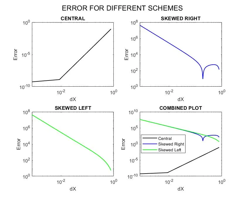
Figure 1: A comparison of the absolute error for different schemes
CONCLUSION:
It could be observed from the above plot in Figure 1 that for both Skewed Left Sided scheme and Skewed Right sided scheme, the error decreases with increase in the step size. In contrast to this the error for the Central Difference scheme increases with increase in step size, as expected. However, for each step size, the absolute error is always the smallest for the Central Difference scheme among all the three schemes.