Week 3.5 - Deriving 4th order approximation of a 2nd order derivative using Taylor Table method
SKEWED RIGHT SIDED DIFFERNCE 4TH ORDER APPROXIMATION OF A 2ND ORDER DERIVATIVE
P = N - Q
where,
P - order of accuracy
N - no. of nodes
Q - order of derivatives f
wkt, P = 4, Q = 2
N = P + Q
N = 4 + 2
N = 6

Derivation:
To derive a fourth order approximation for the second order derivative, we start with this approximation
∂2u/∂x2 = (af(i) + bf(i+1) + cf(i+2) + df(i+3) + ef(i+4) + gf(i+5)) / dx2
Taylor series derivation for the above terms:
bf(i+1)
f(i+1) = [f(i)] + [(f'(i) * Δx)/ 1!] + [(f''(i) * (Δx)2)/ 2!] + [(f'''(i) * (Δx)3)/ 3!] + [(f''''(i) * (Δx)4)/ 4!] + [(f'''''(i) * (Δx)5)/ 5!] + [(f''''''(i) * (Δx)6)/ 6!]
f(i+1) = [f(i)] + [(f'(i) * Δx)/ 1] + [(f''(i) * (Δx)2)/ 2] + [(f'''(i) * (Δx)3)/ 6] + [(f''''(i) * (Δx)4)/ 24] + [(f'''''(i) * (Δx)5)/ 120] + [(f''''''(i) * (Δx)6)/ 720]
multiply by b on both sides
bf(i+1) = [bf(i)] + [(bf'(i) * Δx)/ 1] + [(bf''(i) * (Δx)2)/ 2] + [(bf'''(i) * (Δx)3)/ 6] + [(bf''''(i) * (Δx)4)/ 24] + [(bf'''''(i) * (Δx)5)/ 120] + [(bf''''''(i) * (Δx)6)/ 720]
same procedure for all the terms in the equation:
cf(i+2) = [cf(i)] + [(cf'(i) * 2Δx)/ 1] + [(cf''(i) * 4Δx2)/ 2] + [(cf'''(i) * 8Δx3)/ 6] + [(cf''''(i) * 16Δx4)/ 24] + [(cf'''''(i) * 32Δx5)/ 120] + [(cf''''''(i) * 64Δx6)/ 720]
df(i+3) = [df(i)] + [(df'(i) * 3Δx)/ 1] + [(df''(i) * 9Δx2)/ 2] + [(df'''(i) * 27Δx3)/ 6] + [(df''''(i) * 81Δx4)/ 24] + [(df'''''(i) * 243Δx5)/ 120] + [(df''''''(i) * 729Δx6)/ 720]
ef(i+4) = [ef(i)] + [(ef'(i) * 4Δx)/ 1] + [(ef''(i) * 16Δx2)/ 2] + [(ef'''(i) * 64Δx3)/ 6] + [(ef''''(i) * 256Δx4)/ 24] + [(ef'''''(i) * 1024Δx5)/ 120] + [(ef''''''(i) * 4096Δx6)/ 720]
gf(i+5) = [gf(i)] + [(gf'(i) * 5Δx)/ 1] + [(gf''(i) * 25Δx2)/ 2] + [(gf'''(i) * 125Δx3)/ 6] + [(gf''''(i) * 625Δx4)/ 24] + [(gf'''''(i) * 3125Δx5)/ 120] + [(gf''''''(i) * 15625Δx6)/ 720]
Taylors table:
| f(i) | Δx * f'(i) | Δx2 * f''(i) | Δx3 * f'''(i) | Δx4 * f''''(i) | Δx5 * f'''''(i) | Δx6 * f''''''(i) | |
| af(i) | a | 0 | 0 | 0 | 0 | 0 | 0 |
| bf(i+1) | b | b | b/2 | b/6 | b/24 | b/120 | b/720 |
| cf(i+2) | c | 2c | 4c/2 | 8c/6 | 16c/24 | 32c/120 | 64c/720 |
| df(i+3) | d | 3d | 9d/2 | 27d/6 | 81d/24 | 243d/120 | 729d/720 |
| ef(i+4) | e | 4e | 16e/2 | 64e/6 | 256e/24 | 1024e/120 | 4096e/720 |
| gf(i+5) | g | 5g | 25g/2 | 125g/6 | 625g/24 | 3125g/120 | 15625g/720 |
| 0 | 0 | 1 | 0 | 0 | 0 | ? |
Why there is 0, 1 and '?'
- as we are trying to complete second order derivative, so the only term needs to have is f''.
- other column will be as 0
- because the functions have only 5 terms, we don't know the value for 6th term. hence '?' is given
a + b + c +d + e + g = 0 ----- 1
0 + b + 2c + 3d + 4e + 5g = 0 ----- 2
0 + b/2 + 4c/2 + 9d/2 + 16e/2 + 25g/2 = 1 ----- 3
0 + b/6 + 8c/6 + 27d/6 + 64e/6 + 125g/6 = 0 ----- 4
0 + b/24 + 16c/24 + 81d/24 + 256e/24 + 625g/24 = 0 ----- 5
0 + b/120 + 32c/120 + 243d/120 + 1024e/120 + 3125g/120 = 0 ----- 6
Rearranging into matrix form:
A = [1,1,1,1,1,1;0,1,2,3,4,5;0,1/2,2,9/2,16/2,25/2;0,1/6,8/6,27/6,64/6,125/6;0,1/24,16/24,81/24,256/24,625/24;0,1/120,32,243/120,1024/120,3125/120]
B = [0;0;1;0;0;0]
X = [a,b,c,d,e,g]
X = B/A
from solving in Matlab, we get
a = 3.75
b = 12.8333
c = 17.8333
d = -13.000
e = 5.0833
g = -0.8333
The equation for skewed right-side difference fourth order approximation using second order derivative using Taylor series will be
∂2u/∂x2 = (3.75*f(i) -12.8333*f(i+1) + 17.8333*f(i+2) - 13.000*f(i+3) + 5.08333*f(i+4) -0.8333*f(i+5)) / dx2
SKEWED LEFTSIDED DIFFERNCE 4TH ORDER APPROXIMATION OF A 2ND ORDER DERIVATIVE
P = N - Q
where,
P - order of accuracy
N - no. of nodes
Q - order of derivatives f
wkt, P = 4, Q = 2
N = P + Q
N = 4 + 2
N = 6

Derivation:
To derive a fourth order approximation for the second order derivative, we start with this approximation
∂2u/∂x2 = (af(i-5) + bf(i-4) + cf(i-3) + df(i-2) + ef(i-1) + gf(i)) / dx2
Taylor series derivation for the above terms:
ef(i-1) = [ef(i)] - [(ef'(i) * Δx)/ 1] + [(ef''(i) * (Δx)2)/ 2] - [(ef'''(i) * (Δx)3)/ 6] + [(ef''''(i) * (Δx)4)/ 24] - [(ef'''''(i) * (Δx)5)/ 120] + [(ef''''''(i) * (Δx)6)/ 720]
df(i-2) = [df(i)] - [(df'(i) * 2Δx)/ 1] + [(df''(i) * 4Δx2)/ 2] - [(df'''(i) * 8Δx3)/ 6] + [(df''''(i) * 16Δx4)/ 24] - [(df'''''(i) * 32Δx5)/ 120] + [(df''''''(i) * 64Δx6)/ 720]
cf(i-3) = [cf(i)] - [(cf'(i) * 3Δx)/ 1] + [(cf''(i) * 9Δx2)/ 2] - [(cf'''(i) * 27Δx3)/ 6] + [(cf''''(i) * 81Δx4)/ 24] - [(cf'''''(i) * 243Δx5)/ 120] + [(cf''''''(i) * 729Δx6)/ 720]
bf(i-4) = [bf(i)] - [(bf'(i) * 4Δx)/ 1] + [(bf''(i) * 16Δx2)/ 2] - [(bf'''(i) * 64Δx3)/ 6] + [(bf''''(i) * 256Δx4)/ 24] - [(bf'''''(i) * 1024Δx5)/ 120] + [(bf''''''(i) * 4096Δx6)/ 720]
af(i-5) = [af(i)] - [(af'(i) * 5Δx)/ 1] + [(af''(i) * 25Δx2)/ 2] - [(af'''(i) * 125Δx3)/ 6] + [(af''''(i) * 625Δx4)/ 24] - [(af'''''(i) * 3125Δx5)/ 120] + [(af''''''(i) * 15625Δx6)/ 720]
Taylors table:
| f(i) | Δx * f'(i) | Δx2 * f''(i) | Δx3 * f'''(i) | Δx4 * f''''(i) | Δx5 * f'''''(i) | Δx6 * f''''''(i) | |
| af(i-5) | a | -5a | 25a/2 | -125a/6 | 625a/24 | -3125a/120 | 15625a/720 |
| bf(i-4) | b | -4b | 16b/2 | -64b/6 | 256b/24 | -1024b/120 | 4096b/720 |
| cf(i-3) | c | -3c | 9c/2 | -27c/6 | 81c/24 | -243c/120 | 729c/720 |
| df(i-2) | d | -2d | 4d/2 | -8d/6 | 16d/24 | -32d/120 | 64d/720 |
| ef(i-1) | e | -e | e/2 | -e/6 | e/24 | -e/120 | e/720 |
| gf(i) | g | 0 | 0 | 0 | 0 | 0 | 0 |
| 0 | 0 | 1 | 0 | 0 | 0 | ? |
a + b + c + d + e + g = 0 ----- 1
- 5a - 4b - 3c - 2d - e + 0 = 0 ----- 2
25a/2 + 16b/2 + 9c/2 + 4d/2 + e/2 + 0 = 1 ----- 3
-125a/6 - 64b/6 - 27c/6 -8d/6 - e/6 + 0 = 0 ----- 4
625a/24 + 256b/24 + 81c/24 + 16d/24 + e/24 + 0 = 0 ----- 5
-3125a/120 - 1024b/120 - 243c/120 - 32d/120 - e/120 + 0 = 0 ----- 6
Rearranging into matrix form:
A = [1,1,1,1,1,1;-5,-4,-3,-2,-1,0;25/2,16/2,9/2,4/2,1/2,0;-125/6,-64/6,-27/6,-8/6,-1/6,0;625/24,256/24,81/24,16/24,1/24,0;-3125/120,-1024/120,-243/120,-32/120,-1/120,0]
B = [0;0;1;0;0]
X = [a,b,c,d,e,g]
X = B/A
from solving in Matlab, we get
a = -0.8333
b = 5.0833
c = -13.000
d = 17.8333
e = -12.8333
g = 3.7500
The equation for skewed left-side difference fourth order approximation using second order derivative using Taylor series will be
∂2u/∂x2 = (-0.8333*f(i-5) -5.0833*f(i-4) -13.000*f(i-3) +17.8333*f(i-2) -12.8333*f(i-1) +3.7500*f(i)) / dx2
CENTRAL DIFFERNCE 4TH ORDER APPROXIMATION OF A 2ND ORDER DERIVATIVE
P = N - Q + 1
where,
P - order of accuracy
N - no. of nodes
Q - order of derivatives f
wkt, P = 4, Q = 2
N = P + Q - 1
N = 4 + 2 - 1
N = 5

Derivation:
To derive a fourth order approximation for the second order derivative, we start with this approximation
∂2u/∂x2 = (af(i-2) + bf(i-1) + cf(i) + df(i+1) + ef(i+2)) / dx2
Taylors table:
| f(i) | Δx * f'(i) | Δx2 * f''(i) | Δx3 * f'''(i) | Δx4 * f''''(i) | Δx5 * f'''''(i) | Δx6 * f''''''(i) | |
| af(i-2) | a | -2a | 4a/2 | -8a/6 | 16a/24 | -32a/120 | 64a/720 |
| bf(i-1) | b | -b | b/2 | -b/6 | b/24 | -b/120 | b/720 |
| cf(i) | c | 0 | 0 | 0 | 0 | 0 | 0 |
| df(i+1) | d | d | d/2 | d/6 | d/24 | d/120 | d/720 |
| ef(i+2) | e | 2e | 4e/2 | 8e/6 | 16e/24 | 32e/120 | 64e/720 |
| 0 | 0 | 1 | 0 | 0 | ? | ? |
a + b + c + d + e + g = 0 ----- 1
-2a - b + 0 + d + 2e = 0 ----- 2
2a + b/2 + 0 + d/2 + 2e = 1 ----- 3
-8a/6 - b/6 + 0 + d/6 + 8e/6 = 0 ----- 4
16a/24 + b/24 + 0 + d/24 + 16e/24 = 0 ----- 5
Rearranging into matrix form:
A = [1,1,1,1,1;-2,-1,0,1,2;2,1/2,0,1/2,2;-8/6,-1/6,0,1/6,8/6;16/24,1/24,0,1/24,16/24]
B = [0;0;1;0;0]
X = [a,b,c,d,e]
X = B/A
from solving in Matlab, we get
a = -0.8333
b = 1.333
c = -2.500
d = 1.333
e = -0.0833
The equation for central difference fourth order approximation using second order derivative using Taylor series will be
∂2u/∂x2 = (-0.8333*f(i-2) +1.333*f(i-1) -2.5000*f(i) +1.333*f(i+1) -0.0833*f(i+2)) / dx2
MATLAB CODE
CODE EXPLANATION:
this Matlab script calculates and analyses the numerical second derivative of the function f(x) = ex * cos(x) using three schemes: left skewed, central differencing and right skewed.
it compares the errors in theses numerical methods against the analytical second derivative,
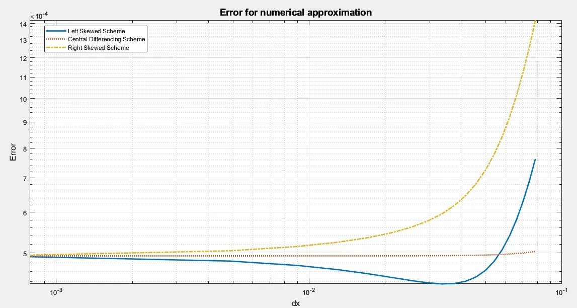
The graph shows the error for numerical approximation of the second derivative of the function
f(x)=exp(x)cos(x) using different numerical schemes (skewed left, central differencing, and skewed right) against varying values of
dx. Here's a detailed explanation of the graph:
Graph Analysis:
Axes:
- X-axis: The values of dx, which represent the step size or grid spacing used in the numerical approximation. These values are plotted on a logarithmic scale.
- Y-axis: The magnitude of the error between the numerical second derivative and the exact (analytical) second derivative. It’s also plotted on a logarithmic scale.
Lines in the Graph:
- Blue line (Left Skewed Scheme): This represents the error in the left-skewed numerical approximation of the second derivative. The error starts to grow sharply as dx increases.
- Orange line (Central Differencing Scheme): This represents the error in the central differencing approximation. The error remains relatively smaller compared to the skewed schemes, indicating better accuracy for a larger range of dx
- Yellow line (Right Skewed Scheme): This represents the error in the right-skewed numerical approximation. The error grows even more rapidly compared to the left-skewed scheme as dx increases.
Key Observations:
Error Magnitude:
- For small dx values, the central differencing scheme produces the smallest error, which is expected since it has a higher order of accuracy (i.e. O(h^4))
- dx increases, the errors in both skewed schemes (left and right) grow significantly, especially the right-skewed scheme, due to the lower order of truncation error and sensitivity to rounding errors.
Error Growth:
- In the graph, the error for the skewed schemes increases sharply as dx moves toward higher values.
- This suggests that these schemes are sensitive to the step size and their accuracy worsens as dx becomes larger.
- The central differencing scheme exhibits relatively stable error growth, making it more accurate for a wide range of
.
Truncation Error Comparison:
- The central differencing scheme has a truncation error of O(h^4) meaning that the error decreases at a rate proportional to dx^4
- This explains why its error grows slower for small dx.
- On the other hand, the skewed schemes have truncation errors of O(h^6) meaning they are theoretically more accurate (error decreases faster with decreasing dx), but in practice, they are more prone to round-off errors, especially for small dx.
Logarithmic Scale:
- The use of log-log scales (for both axes) helps to visualize the error growth at different magnitudes of dx.
- This makes it easier to compare the rates at which the errors increase for different schemes.
Conclusion:
- The central differencing scheme is the most reliable in terms of error for a wide range of dx, providing stable and accurate results.
- The left and right skewed schemes offer better theoretical accuracy (since their truncation error is of order, but they become less accurate due to round-off errors as dx becomes very small.
- For practical purposes, central differencing is preferred because it offers a good balance between accuracy and stability, especially when dx is not too small.