Week 3.5 - Deriving 4th order approximation of a 2nd order derivative using Taylor Table method

The aim of this assignment is to write a program in MATLAB to derive the fourth order approximations of the second order derivative of "exp(x)*cos(x)" utilising the Taylor's table and to compare the results of the approximations against the analytically computed value of the derivative and visualise the error that each of these schemes yield in the form of a loglog curve between the "absolute error" and "dx".

Developing the schemes:

Central Difference:

Taylor's table:

	`f(i)`	`f'(i)*Deltax`	`f''(i)*Deltax^2`	`f'''(i)*Deltax^3`	`f^(iv)(i)*Deltax^4`	`f^(v)(i)*Deltax^5`	`f^(vi)(i)*Deltax^6`
afi-2	a	-2a/1!=2a	4a/2!=2a	-8a/3!=-4a/3	16a/4!=2a/3	-32a/5!=-4a/15	64a/6!=4a/45
bfi-1	b	-b	b/2	-b/6	b/24	-b/120	b/720
cfi	c	0	0	0	0	0	0
dfi+1	d	d	d/2	d/6	d/24	d/120	d/720
efi+2	e	2e	2e	4e/3	2e/3	4e/15	4a/45
SUM:	0	0	1	0	0	---	---

`(del^2f)/(delx^2)`=af_i-2+bf_i-1+cf_i+df_i+1+ef_i+2

a+b+c+d+e=0

-2a-b+0+d+2e=0

2a+b/2+0+d/2+2e=1

-4a/3-b/6+0+d/6+4e/3=0

2a/3+b/24+0+d/24+2e/3=0

The code:

clear
close all
clc
%Let the coefficient matrix be A, the matrix of constants be B
%The solution matrix is X;
A=[1 1 1 1 1;-2 -1 0 1 2;2 1/2 0 1/2 2; -4/3 -1/6 0 1/6 4/3;2/3 1/24 0 1/24 2/3];
B=[0 0 1 0 0]';
%By method of matrix multiplication:
X=inv(A)*B;

Obtained value of solution vector:

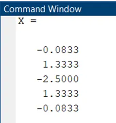
a=e=-0.0833

b=d=1.3333

c=-2.5

To show that it is fourth order accurate:

`(del^2f)/(delx^2)=`af_i-2+bf_i-1+cf_i+df_i+1+ef_{i+2 .....(Hypothesis function)}

`(del^2f)/(delx^2)=`f(i)(a+b+c+d+e)+f'(i)`Deltax`(-2a-b+d+2e)+f"(i)`Deltax^2`(2a+b/2+d/2+2e)

f'''(i)`Deltax^3`(-4a/3-b/6+d/6+4e/3)+`f^(iv)(i)Deltax^4`(2a/3+b/24+d/24+2e/3)

`f^(v)(i)Deltax^5`(-4a/15-b/120+d/120+4e/15)+`f^(vi)(i)Deltax^6`(4a/45+b/720+d/720+

4e/45)+...

`(del^2f)/(delx^2)=`f(i)*0+f'(i)`Deltax`*0+f"(i)`Deltax^2`*1+f'''(i)`Deltax^3`*0+`f^(iv)(i)Deltax^4`*0+

`f^(v)(i)Deltax^5`(-4a/15-b/120+d/120+4e/15)+`f^(vi)(i)Deltax^6`(4a/45+b/720+d/720+

4e/45)+...

as a=e and b=d;

`(del^2f)/(delx^2)=`f"(i)`Deltax^2`+`f^(v)(i)Deltax^5`*0+`f^(vi)(i)Deltax^6`*(non zero value)

f"(i) is the approximation (taking only the first 5 terms in the taylor series expansion);

`(del^2f)/(delx^2)=``(f''(i)+o(Deltax^4))/(Deltax^2)`

Thus the error is of the fourth order.

Skewed Right-Sided Difference:

Taylor's table:

	`f(i)`	`f'(i)*Deltax`	`f''(i)*Deltax^2`	`f'''(i)*Deltax^3`	`f^(iv)(i)*Deltax^4`	`f^(v)(i)*Deltax^5`	`f^(vi)(i)*Deltax^6`
afi	a	0	0	0	0	0	0
bfi+1	b	b	b/2	b/6	b/24	b/120	b/720
cfi+2	c	2c	2c	4/3c	2/3c	4/15c	4/45
dfi+3	d	3d	9d/2	9d/2	27d/8	81d/40	81d/80
efi+4	e	4e	8e	32e/3	32e/3	128e/15	256e/45
gfi+5	g	5g	25g/2	126g/6	625g/24	625g/24	3125g/144
SUM:	0	0	1	0	0	0	---

`(del^2f)/(delx^2)`=af_i+bf_i+1+cf_i+2+df_i+3+ef_i+4+gf_{i+5 ...(Hypothesis Function)}

Solving for a,b,c,d,e,g as done earlier (by matrix inversion method)

Code:

clear
close all
clc
%Let the coefficient matrix be A, the matrix of constants be B
%The solution matrix is X;
A=[1 1 1 1 1 1;0 1 2 3 4 5;0 1/2 2 9/2 8 25/2;0 1/6 4/3 9/2 32/3 125/6;0 1/24 2/3 27/8 32/3 625/24;0 1/120 4/15 81/40 128/15 625/24];
B=[0 0 1 0 0 0]';
%By method of matrix multiplication:
X=inv(A)*B;

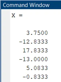
Obtained value of solution vector:

`(del^2f)/(delx^2)=`af_i+bf_i+1+cf_i+2+df_i+3+ef_i+4 +gf_{i+5 .....(Hypothesis function)}

`(del^2f)/(delx^2)=`f(i)*0+f'(i)`Deltax`*0+f''(i)`Deltax^2`*1+f'''(i)`Deltax^3`+`f^(iv)Deltax^4`*0+`f^(v)Deltax^5`*0+`f^(vi)Deltax^6`*(non zero value)

f"(i) is the approximation (taking only the first 6 terms in the taylor series expansion);

`(del^2f)/(delx^2)=``(f''(i)+o(Deltax^4))/(Deltax^2)`

Thus the error is of the fourth order.

Skewed Left-Sided Difference:

Taylor's table:

	`f(i)`	`f'(i)*Deltax`	`f''(i)*Deltax^2`	`f'''(i)*Deltax^3`	`f^(iv)(i)*Deltax^4`	`f^(v)(i)*Deltax^5`	`f^(vi)(i)*Deltax^6`
afi	a	0	0	0	0	0	0
bfi-1	b	-b	b/2	-b/6	b/24	-b/120	b/720
cfi-2	c	-2c	2c	-4/3c	2/3c	-4/15c	4/45
dfi-3	d	-3d	9d/2	-9d/2	27d/8	-81d/40	81d/80
efi-4	e	-4e	8e	-32e/3	32e/3	-128e/15	256e/45
gfi-5	g	-5g	25g/2	-126g/6	625g/24	-625g/24	3125g/144
SUM:	0	0	1	0	0	0	---

`(del^2f)/(delx^2)`=af_i+bf_i-1+cf_i-2+df_i-3+ef_i-4+gf_{i-5 ...(Hypothesis Function)}

Solving for a,b,c,d,e,g as done earlier (by matrix inversion method)

Code:

clear
close all
clc
%Let the coefficient matrix be A, the matrix of constants be B
%The solution matrix is X;
A=[1 1 1 1 1 1;0 -1 -2 -3 -4 -5;0 1/2 2 9/2 8 25/2;0 -1/6 -4/3 -9/2 -32/3 -125/6;0 1/24 2/3 27/8 32/3 625/24;0 -1/120 -4/15 -81/40 -128/15 -625/24];
B=[0 0 1 0 0 0]';
%By method of matrix multiplication:
X=inv(A)*B;

The solution vector:

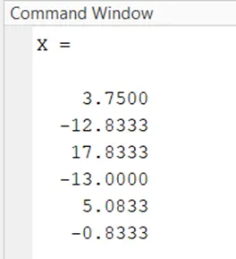
The proof that the accuracy for this scheme is of the fourth order is the same as for the right sided skewness scheme.

Central Difference Scheme:

`f''(x)=(-0.0833f(x-2*dx)+1.3333*f(x-dx)-2.5*f(x)+1.3333*f(x+dx)-0.0833f(x+2*dx))/dx^2`

Skewed Right-Sided Scheme:

`f''(x)=(3.75*f(x)-12.8333*f(x+dx)+17.8333f(x+2*dx)-13*f(x+3*dx)+5.0833*f(x+4*dx)-0.8333f(x+5*dx))/dx^2`

Skewed Left-Sided Scheme:

`f''(x)=(3.75*f(x)-12.8333*f(x-dx)+17.8333f(x-2*dx)-13*f(x-3*dx)+5.0833*f(x-4*dx)-0.8333f(x-5*dx))/dx^2`

Using the obtained coefficients, a code was written in MATLAB to plot the errors from the different schemes against the values of "dx".

MAIN CODE for computing the accuracy:

clear
close all
clc
x=pi/3;
dx=linspace(pi/3000,pi/3,20);
%given function: f(x)=exp(x)*cos(x);
%analytical_derivative=-exp(x)*(cos(x)+sin(x))
analytical_derivative=-2*exp(x)*sin(x);
for i=1:20
%central_difference=(-0.0833f(x-2*dx)+1.3333*f(x-dx)-2.5*f(x)+1.3333*f(x+dx)-0.0833f(x+2*dx))/dx^2
%right_skewed=(3.75*f(x)-12.8333*f(x+dx)+17.8333f(x+2*dx)-13*f(x+3*dx)+5.0833*f(x+4*dx)-0.8333f(x+5*dx))/dx^2
%left_skewed=(3.75*f(x)-12.8333*f(x-dx)+17.8333f(x-2*dx)-13*f(x-3*dx)+5.0833*f(x-4*dx)-0.8333f(x-5*dx))/dx^2
%Coefficients for central_difference:
A=[1 1 1 1 1;-2 -1 0 1 2;2 1/2 0 1/2 2;-4/3 -1/6 0 1/6 4/3;2/3 1/24 0 1/24 2/3];
B=[0 0 1 0 0 ]';
%By method of matrix multiplication:
X=inv(A)*B;
%Coefficients for right_skewed
A1=[1 1 1 1 1 1;0 1 2 3 4 5;0 1/2 2 9/2 8 25/2;0 1/6 4/3 9/2 32/3 125/6;0 1/24 2/3 27/8 32/3 625/24;0 1/120 4/15 81/40 128/15 625/24];
B1=[0 0 1 0 0 0]';
%By method of matrix multiplication:
X1=inv(A1)*B1;
%Coefficients for left_skewed
A2=[1 1 1 1 1 1;0 -1 -2 -3 -4 -5;0 1/2 2 9/2 8 25/2;0 -1/6 -4/3 -9/2 -32/3 -125/6;0 1/24 2/3 27/8 32/3 625/24;0 -1/120 -4/15 -81/40 -128/15 -625/24];
B2=[0 0 1 0 0 0]';
%By method of matrix multiplication:
X2=inv(A2)*B2;
central_difference(i)=(X(1)*exp(x-2*dx(i))*cos(x-2*dx(i))+X(2)*exp(x-dx(i))*cos(x-dx(i))+X(3)*exp(x)*cos(x)+X(4)*exp(x+dx(i))*cos(x+dx(i))+X(5)*exp(x+2*dx(i))*cos(x+2*dx(i)))/dx(i)^2;
right_skewed(i)=(X1(1)*exp(x)*cos(x)+X1(2)*exp(x+dx(i))*cos(x+dx(i))+X1(3)*exp(x+2*dx(i))*cos(x+2*dx(i))+X1(4)*exp(x+3*dx(i))*cos(x+3*dx(i))+X1(5)*exp(x+4*dx(i))*cos(x+4*dx(i))+X1(6)*exp(x+5*dx(i))*cos(x+5*dx(i)))/dx(i)^2;
left_skewed(i)=(X2(1)*exp(x)*cos(x)+X2(2)*exp(x-dx(i))*cos(x-dx(i))+X2(3)*exp(x-2*dx(i))*cos(x-2*dx(i))+X2(4)*exp(x-3*dx(i))*cos(x-3*dx(i))+X2(5)*exp(x-4*dx(i))*cos(x-4*dx(i))+X2(6)*exp(x-5*dx(i))*cos(x-5*dx(i)))/dx(i)^2;
end
error_central_difference=abs(central_difference-analytical_derivative);
error_right_skewed=abs(right_skewed-analytical_derivative);
error_left_skewed=abs(left_skewed-analytical_derivative);
figure(1)
title('loglog plot for error-vs-dx')
loglog(dx,error_central_difference,'r')
hold on
loglog(dx,error_right_skewed,'g')
hold on
loglog(dx,error_left_skewed,'b')
legend('Red-> Central Difference','Green->Right Skewed','Blue->Left Skewed')
xlabel('dx');
ylabel('absolute error')

Results and Inferences:

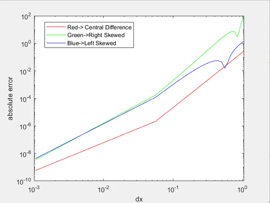
The central differencing scheme yields the least error.

As the value of 'dx' increases, the error increases exponentially for all the schemes, however, it is more pronounced in the skewed schemes.

***Why are the Skewed schemes are useful?

Despite yielding greater error (as can be observed above) and being computationally expensive, the skewed schemes are sometimes deemed better.

They are the preferred mode of dicretisation when the flow direction is not aligned with the grid lines.

For example, in modelling linear convection, the skewed schemes are chosen over central differencing schemes, despite being more accurate, as they can introduce numerical oscillations and false diffusion causing the solution to "blow up".