Week 3.5 - Deriving 4th order approximation of a 2nd order derivative using Taylor Table method

AIM:Derive the following 4th order approximations of the second-order derivative.

1. Central difference

2. Skewed right-sided difference

3. Skewed left-sided difference

Objective:

Derive the Central difference 4th order approximations of the second-order derivative.

Derive the Skewed right-sided difference 4th order approximations of the second-order derivative.

Derive the Skewed left-sided difference4th order approximations of the second-order derivative.

Write a program in Matlab to evaluate the second-order derivative of a given analytical function using all three 4th order approximation schemes.

Compare the results obtained in three approximation schemes.

Provide a plot that compares the absolute error between the above-mentioned schemes.

describe why a skewed scheme is useful and what can a skewed scheme do that a CD scheme cannot?

Skewed right-sided difference:

Number of nodes in the stencil (N)=The order of accuracy P + order of derivative Q

N=4+2=6

Lt's consider the equation of second derivative of a function at ith node using using scewed right side difference scheme is as follows:

`(del^2f)/ (del x^2)cong(delta^2f)/(deltax^2)`=a*f(i)+b*f(i+1)+c*f(i+2)+d*f(i+3)+e*f(i+4)+f*f(i+5).......eq(1)

Now expanding each term we get-

a*f(i)=a*f(i)

b*f(i+1) =b[`f(i)+(Deltax)/1*f'(i)+(Deltax)^2/2*f''(i)+(Deltax)^3/6*f'''(i)+(Deltax)^4/24*f^(iv)(i)+(Deltax)^5/120*f^v(i)+(Deltax)^6/720*f^(vi)(i)`]`

c*f(i+2)=`c[f(i)+(2Deltax)/1*f'(i)+(2Deltax)^2/2*f''(i)+(2Deltax)^3/6*f'''(i)+(2*Deltax)^4/24*f^(iv)(i)+(2*Deltax)^5/120*f^v(i)+(2*Deltax)^6/720*f^(vi)(i)`]`

d*f(i+3)=`d[f(i)+(3Deltax)/1*f'(i)+(3Deltax)^2/2*f''(i)+(3Deltax)^3/6*f'''(i)+(3Deltax)^4/24*f^(iv)(i)+(3Deltax)^5/120*f^v(i)+(3Deltax)^6/720*f^(vi)(i)`]`

e*f(i+4)=`e[f(i)+(4Deltax)/1*f'(i)+(4Deltax)^2/2*f''(i)+(4Deltax)^3/6*f'''(i)+(4Deltax)^4/24*f^(iv)(i)+(4Deltax)^5/120*f^v(i)+(4Deltax)^6/720*f^(vi)(i)`]`

f*f(i+5)=`f[f(i)+(5Deltax)/1*f'(i)+(5Deltax)^2/2*f''(i)+(5Deltax)^3/6*f'''(i)+(5Deltax)^4/24*f^(iv)(i)+(5Deltax)^5/120*f^v(i)+(5Deltax)^6/720*f^(vi)(i)`]`

Putting these values in equation 1 we get....

`(del^2f)/ (del x^2)cong`(a+b+c+d+e+f)f(i)+`(b+2c+3d+4e+5f)Deltaxf'(i)``+(`(b/2+2c+(9d)/2+8e+(25f)/2)(Delta x)^2f''(i)``+`(b/6+4/3c+9/2d+32/3e+125/6f)(Deltax)^3f'''(i)`+`(b/24+2/3c+27/8d+32/3e+625/24f)(Deltax)^4f^iv(i)`+`b/120+32/120c+243/120d+128/15e+625/24f)(Deltax)^5f^v(i)`+`(b/720+4/45c+81/80d+256/45e+3125/144f)(Deltax)^6f^(vi)(i)` eq.(2)

In Eq(2) coefficients of f''(i) is equals to 1 and coefficients of rest of derivative terms are zero.Hence we get equations as follows.

a+b+c+d+e+f=0

b+2c+3d+4e+5f=0

b/2+2c+(9d)/2+8e+(25f)/2=1

b/6+4/3c+9/2d+32/3e+125/6f=0

b/24+2/3c+27/8d+32/3e+625/24f=0

b/120+32/120c+243/120d+128/15e+625/24f=0

b/720+4/45c+81/80d+256/45e+3125/144f=0

Writing these coefficient in table format is called as Taylor's table

Taylor's Table

	f(i)	`(Deltax)f'(i)`	`(Deltax)^2f''(i)`	`(Deltax)^3f'''(i)`	`(Deltax)^4f^iv(i)`	`(Deltax)^5f^v(i)`	`(Deltax)^6f^(vi)(i)`
af(i)	a	0	0	0	0	0	0
bf(i+1)	b	b	b/2	b/6	b/24	b/120	b/720
cf(i+2)	c	2c	2c	4c/3	2c/3	32c/120	4c/45
df(i+3)	d	3d	9d/2	9d/2	27d/8	243d/120	81d/80
ef(i+4)	e	4e	8e	32e/3	32e/3	128e/15	256e/45
ff(i+5)	f	5f	25f/2	125f/6	625f/24	625f/24	3125f/144
	0	0	1	0	0	0	0

Putting them in matrix form we get-

`[ [1,1,1,1,1,1], [ 0,1,2,3,4,5] ,[ 0,1/2,2,9/2,8,25/2],[ 0,1/6,4/3,9/2,32/3,125/6],[ 0,1/24,2/3,27/8,32/3,625/24],[0,1/120,32/120,243/120,128/15,625/24] ][[a],[b],[c],[d],[e],[f]]=[[0],[0],[1],[0],[0],[0]]`

solving the avove system of linear equations in matlab we get

`[[a],[b],[c],[d],[e],[f]]=[[3.7500],[-12.8333],[17.8333 ],[-13.0000],[ 5.0833],[-0.8333]]`

hence final second order derivation expression is-

`(del^2f)/ (del x^2)cong(delta^2f)/(deltax^2)=(3.75*f(i)-12.8333*f(i+1)+17.8333*f(i+2)-13*f(i+3)+5.08330*f(i+4)-0.83330*f(i+5))/(Deltax)^2``

Central difference:Here for symmetric/central scheme

Number of nodes in the stencil (N)=The order of accuracy P + order of derivative Q - 1

N=4+2-1=5

Lt's consider the equation of second derivative of a function at ith node using using central difference scheme is as follows:

`(del^2f)/ (del x^2)cong(delta^2f)/(deltax^2)`=a*f(i)+b*f(i-2)+c*f(i-1)+d*f(i+1)+e*f(i+2) .eq(3)

af(i)=af(i)

b*f(i-2)=`b[f(i)-(2Deltax)/1*f'(i)+(2Deltax)^2/2*f''(i)-(2Deltax)^3/6*f'''(i)+(2*Deltax)^4/24*f^(iv)(i)-(2*Deltax)^5/120*f^v(i)+(2*Deltax)^6/720*f^(vi)(i)`]`

c*f(i-1)=`c[f(i)-(Deltax)/1*f'(i)+(Deltax)^2/2*f''(i)-(Deltax)^3/6*f'''(i)+(Deltax)^4/24*f^(iv)(i)-(Deltax)^5/120*f^v(i)+(Deltax)^6/720*f^(vi)(i)``

d*f(i+1)=`d[f(i)+(2Deltax)/1*f'(i)+(2Deltax)^2/2*f''(i)+(2Deltax)^3/6*f'''(i)+(2*Deltax)^4/24*f^(iv)(i)+(2*Deltax)^5/120*f^v(i)+(2*Deltax)^6/720*f^(vi)(i)`]`

e*f(i+2)=`e[f(i)+(2Deltax)/1*f'(i)+(2Deltax)^2/2*f''(i)+(2Deltax)^3/6*f'''(i)+(2*Deltax)^4/24*f^(iv)(i)+(2*Deltax)^5/120*f^v(i)+(2*Deltax)^6/720*f^(vi)(i)`]`

Putting these values of x into eq(3) we get

`(del^2f)/ (del x^2)cong`(`(a+b+c+d+e)f(i)``+`(-2b-2c+d+2e)Deltaxf'(i)``+``(2b+c/2+d/2+2e)(Delta x)^2f''(i)`+`(-4/3b-c/6+d/6+4/3e)(Deltax)^3f'''(i)``+`(2/3b+c/24+d/24+2/3e)(Deltax)^4f^iv(i)`+`-32/120b-c/120+d/120+32/120e)(Deltax)^5f^v(i)`+`(64/720b+c/720+d/720+64/720e)(Deltax)^6f^(vi)(i)`` eqn(3)

In Eq(3) coefficients of f''(i) is equals to 1 and coefficients of rest of derivative terms are zero.Hence we get equations as follows.

a+b+c+d+e=0

-2b-2c+d+2e=0

2b+c/2+d/2+2e=1

-4/3b-c/6+d/6+4/3e=0

2/3b+c/24+d/24+2/3e=0

-32/120b-c/120+d/120+32/120e=0

64/720b+c/720+d/720+64/720e=0

`[[ 1,1,1,1,1],[0,-2,-1,1,2],[0,2,1/2,1/2,2],[0,-4/3,-1/6,1/6,4/3],[0,2/3,1/24,1/24,2/3]][[a],[b],[c],[d],[e]]=[[0],[0],[1],[0],[0]]`

`[[a],[b],[c],[d],[e]]= [[-2.5000],[-0.0833],[1.3333],[1.3333],[-0.0833]]`

`(del^2f)/ (del x^2)cong(delta^2f)/(deltax^2)=(-2.5*f(i)-0.0833*f(i-2)+1.333*f(i-1)+1.333*f(i+1)-0.0833*f(i+2))/(Delta x)^2`

Taylor's Table-

	f(i)	`(Deltax)f'(i)`	`(Deltax)^2f''(i)`	`(Deltax)^3f'''(i)`	`(Deltax)^4f^iv(i)`	`(Deltax)^5f^v(i)`	`(Deltax)^6f^(vi)(i)`
af(i)	a	0	0	0	0	0	0
bf(i-2)	b	-2b	2b	-4b/3	2b/3	-32b/120	64b/720
cf(i-1)	c	-c	c/2	-c/6	c/24	-c/120	c/720
df(i+1)	d	d	d/2	d/6	d/24	d/120	d/720
ef(i+2)	e	2e	2e	4e/3	2e/3	32e/120	64e/720
	0	0	1	0	0	0	0

Skewed left-sided difference

Number of nodes in the stencil (N)=The order of accuracy P + order of derivative Q

N=4+2=6

`(del^2f)/ (del x^2)cong(delta^2f)/(deltax^2)`=a*f(i)+b*f(i-1)+c*f(i-2)+d*f(i-3)+e*f(i-4)+f*f(i-5) .......eq(5)

b*f(i-1)=`b[f(i)-(Deltax)/1*f'(i)+(Deltax)^2/2*f''(i)-(Deltax)^3/6*f'''(i)+(Deltax)^4/24*f^(iv)(i)-(Deltax)^5/120*f^v(i)+(Deltax)^6/720*f^(vi)(i)``

c*f(i-2)=`c[f(i)-(2Deltax)/1*f'(i)+(2Deltax)^2/2*f''(i)-(2Deltax)^3/6*f'''(i)+(2*Deltax)^4/24*f^(iv)(i)-(2*Deltax)^5/120*f^v(i)+(2*Deltax)^6/720*f^(vi)(i)`]`

d*f(i-3)=`d[f(i)-(3Deltax)/1*f'(i)+(3Deltax)^2/2*f''(i)-(3Deltax)^3/6*f'''(i)+(3Deltax)^4/24*f^(iv)(i)-(3Deltax)^5/120*f^v(i)+(3Deltax)^6/720*f^(vi)(i)`]`

e*f(i-4)=`e[f(i)-(4Deltax)/1*f'(i)+(4Deltax)^2/2*f''(i)-(4Deltax)^3/6*f'''(i)+(4Deltax)^4/24*f^(iv)(i)-(4Deltax)^5/120*f^v(i)+(4Deltax)^6/720*f^(vi)(i)`]`

f*f(i-5)=`f[f(i)-(5Deltax)/1*f'(i)+(5Deltax)^2/2*f''(i)-(5Deltax)^3/6*f'''(i)+(5Deltax)^4/24*f^(iv)(i)-(5Deltax)^5/120*f^v(i)+(5Deltax)^6/720*f^(vi)(i)`]`

Putting these values of x into eq(5) we get

`(del^2f)/ (del x^2)cong (a+b+c+d+e+f)f(i)-(b+2c+3d+4e+5f)Delta xf'(i)+(b/2+2c+(9d)/2+8e+(25f)/2)(Delta x)^2f''(i)``-(b/6+4/3c+9/2d+32/3e+125/6f)(Deltax)^3f'''(i)+(b/24+2/3c+27/8d+32/3e+625/24f)(Deltax)^4f^iv(i)-(b/120+32/120c+243/120d+128/15e+625/24f)(Deltax)^5f^v(i)`+`(b/720+4/45c+81/80d+256/45e+3125/144f)(Deltax)^6f^(vi)(i)`` eq(6)

In Eq(6) coefficients of f''(i) is equals to 1 and coefficients of rest of derivative terms are zero.Hence we get equations as follows

a+b+c+d+e+f=0

-b-2c-3d-4e-5f=

b/2+2c+(9d)/2+8e+(25f)/2=1

`(b/6+4/3c+9/2d+32/3e+125/6f)=`

b/24+2/3c+27/8d+32/3e+625/24f=0

-(b/120+32/120c+243/120d+128/15e+625/24f)=0

b/720+4/45c+81/80d+256/45e+3125/144f

`[ [1,1,1,1,1,1], [ 0,-1,-2,-3,-4,-5] ,[ 0,1/2,2,9/2,8,25/2],[ 0,-1/6,-4/3,-9/2,-32/3,-125/6],[ 0,1/24,2/3,27/8,32/3,625/24],[0,-1/120,-32/120,-243/120,-128/15,-625/24] ][[a],[b],[c],[d],[e],[f]]=[[0],[0],[1],[0],[0],[0]]`

`[[a],[b],[c],[d],[e],[f]]=[[3.7500],[-12.8333],[17.8333 ],[-13.0000],[ 5.0833],[-0.8333]]`

`(del^2f)/ (del x^2)cong(delta^2f)/(deltax^2)=(3.75*f(i)-12.8333*f(i-1)+17.8333*f(i-2)-13*f(i+3)+5.08330*f(i-4)-0.83330*f(i-5))/(Deltax)^2`

Taylor's Table-

	f(i)	`(Deltax)f'(i)`	`(Deltax)^2f''(i)`	`(Deltax)^3f'''(i)`	`(Deltax)^4f^iv(i)`	`(Deltax)^5f^v(i)`	`(Deltax)^6f^(vi)(i)`
af(i)	a	0	0	0	0	0	0
bf(i-1)	b	-b	b/2	-b/6	b/24	-b/120	b/720
cf(i-2)	c	-2c	2c	-4c/3	2c/3	-32c/120	4c/45
df(i-3)	d	-3d	9d/2	-9d/2	27d/8	-243d/120	81d/80
ef(i-4)	e	-4e	8e	-32e/3	32e/3	-128e/15	256e/45
ff(i-5)	f	-5f	25f/2	-125f/6	625f/24	-625f/24	3125f/144
	0	0	1	0	0	0	0

Programming to solve the matrix of equations:

%Programming to solve the Linear system of Equations

% Equation obtaine in Skewed right-sided difference Approach

%a+b+c+d+e+f=0
%b+2c+3d+4e+5f=0
%b/2+2c+(9d)/2+8e+(25f)/2=1
%b/6+4/3c+9/3d+32/3e+125/6f=0
%b/24+2/3c+27/8d+32/3e+625/24f=0
%b/120+32/120c+243/120d+128/15e+625/24f=0
%b/720+4/45c+81/80d+256/45e+3125/144f=0

% Solving For Coefficient
A_1=[1,1,1,1,1,1;0,1,2,3,4,5;0,1/2,2,9/2,8,25/2;0,1/6,4/3,9/2,32/3,125/6;0,1/24,2/3,27/8,32/3,625/24;0,1/120,32/120,243/120,128/15,625/24];
B_1=[0;0;1;0;0;0];
 X_R=linsolve(A_1,B_1);

% Equation obtaine in central difference Approach


%    a+b+c+d+e=0;
%   -2b-2c+d+2e=0;
%   2b+c/2+d/2+2e=1;
%  -4/3b-c/6+d/6+4/3e=0;
%   2/3b+c/24+d/24+2/3e=0;
%  -32/120b-c/120+d/120+32/120e=0;
%   64/720b+c/720+d/720+64/720e=0;

% Solving For Coefficient
A_2=[ 1,1,1,1,1;0,-2,-1,1,2;0,2,1/2,1/2,2;0,-4/3,-1/6,1/6,4/3;0,2/3,1/24,1/24,2/3];
B_2=[0;0;1;0;0];
 X_C=linsolve(A_2,B_2);

% Equation obtaine in Skewed left-sided difference Approach

%a+b+c+d+e+f=0
%-b-2c-3d-4e-5f=0
%b/2+2c+(9d)/2+8e+(25f)/2=1
%-(b/6+4/3c+9/3d+32/3e+125/6f)=0
%b/24+2/3c+27/8d+32/3e+625/24f=0
%-(b/120+32/120c+243/120d+128/15e+625/24f)=0
%b/720+4/45c+81/80d+256/45e+3125/144f=0

% Solving For Coefficient
A_3=[1,1,1,1,1,1;0,-1,-2,-3,-4,-5;0,1/2,2,9/2,8,25/2;0,-1/6,-4/3,-9/2,-32/3,-125/6;0,1/24,2/3,27/8,32/3,625/24;0,-1/120,-32/120,-243/120,-128/15,-625/24];
B_3=[0;0;1;0;0;0]; 
X_L=linsolve(A_3,B_3);

Programmig to obtain second order derivative of a given function and error plotting

%f(x)=exp(x)*cos(x)
%Analytical_derivative=-2*sin(x)*exp(x)

%Inputs
x=pi/4;
dx=linspace(pi/20,pi/400,200);

%Creating Ananymous function
f=@(x) exp(x)*cos(x);

% Analytical Derivative Second order
%f(x)=exp(x)*cos(x)
%Analytical_derivative=-2*sin(x)*exp(x)

Analytical_derivative=-2*sin(x)*exp(x);



 for i=1:length(dx)

  % Skewed right-sided difference Approximation(Fourth order approximation
    R_approximation(i)=(X_R(1)*f(x)+X_R(2)*f(x+dx(i))+X_R(3)*f(x+2*dx(i))+X_R(4)*f(x+3*dx(i))+X_R(5)*f(x+4*dx(i))+X_R(6)*f(x+5*dx(i)))/(dx(i))^2;
    
   % Skewed central difference Approximation(Fourth order approximation
    C_Aprroximation(i)=(X_C(1)*f(x)+X_C(2)*f(x-2*dx(i))+X_C(3)*f(x-dx(i))+X_C(4)*f(x+dx(i))+X_C(5)*f(x+2*dx(i)))/(dx(i))^2;
   
   % Skewed Light-sided difference Approximation(Fourth order approximation
    L_Approximation(i)=(X_L(1)*f(x)+X_L(2)*f(x-dx(i))+X_L(3)*f(x-2*dx(i))+X_L(4)*f(x-3*dx(i))+X_L(5)*f(x-4*dx(i))+X_L(6)*f(x-5*dx(i)))/(dx(i))^2;

% Absolute Error Calculation

% Error Skewed right-sided difference
    error_R_approximation(i)=abs(Analytical_derivative-R_approximation(i));

% Error Skewed central difference
    error_C_Aprroximation(i)=abs(Analytical_derivative-C_Aprroximation(i));

 % Error Skewed Left-sided difference
    error_L_Approximation(i)=abs(Analytical_derivative-L_Approximation(i));

 end;

 % Error plotting

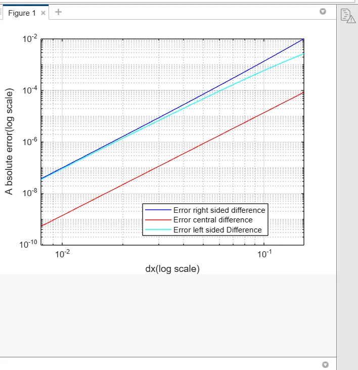
 figure(1)
 loglog(dx,error_R_approximation)
 hold on
 loglog(dx,error_C_Aprroximation)
 hold on
 loglog(dx,error_L_Approximation)
 xlabel('dx(log scale)');
 ylabel('A bsolute error(log scale)');
 legend('Error right sided difference','Error central difference','Error left sided Difference')
    

Code Explanation:

Code Explanation –

Two different programmes is written

First to solve system of linear equations to get coefiiecients of second order derivative expression of fouth order approximation using central and scewed difference schemes.

Second to compute second order derivative of a given function using differen fourth order approximation schemes and plotting error

1. Define the variable x and dx. dx is grid size or we can say approximation distance between two nodes. dx is defined with linspace which provides a range of data.

2.Calling ananymous function given.

3. Define analytical derivative to find second order derivative of given function.

4-Define the R_approximation,C_Aprroximation, L_Approximation, error_R_approximation, error_C_approximation, error_L_approximation variable which is an equation. Define error, which is difference of analytic and numerical derivative.

5. loglog command is used to make log plot in command window.

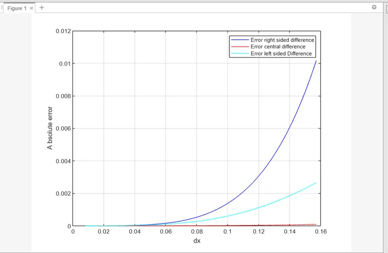
Error plot of three schemes-

Conclusion-

Error is decreasing with decrease in dx value in all three schemes but error for any dx is more in scewed schemes than in central difference sceme .

With decrese in dx value slope is also decreasing.

central difference scheme are good when it comes to comparing error but it can't be used to calculate derivative at extreme left or right nodes or upto some number of nodes in right side and left side of the domain there either of the scewed schemes are useful.