Week 3.5 - Deriving 4th order approximation of a 2nd order derivative using Taylor Table method
AIM:
To derive the fourth order approximations of a second order derivative using central differencing scheme, skewed right sided difference and skewed left sided difference with the help of taylor table method and to compare the analytical derivative with obtained values for the given function.
SCHEME DERIVATIONS:
CENTRAL DIFFERENCING SCHEME:
NO OF NODES:
The number of nodes = p+q-1
Where, p is order of derivative.
q is order of approximations.
The no of nodes = 2+4-1 =>5.
To derive a fourth order approximation for the second order derivative,we start with these approximation,
((del^2(u))/(del(x)^2)) = (af(i-2) + bf(i-1) + cf(i) +df(i+1) + ef(i+2))/x^2..................................1
taylor series derivation for the above terms,
`af(i-2) = f(i) - 2af'(i)dx + (4af''(i)*dx^2)/2 - (8af'''(i)*dx^3)/6 +(16af''''(i)*(dx^4))/24....................................2
Simillarly expand all the terms in the equation (1) and are represented in the form of table using taylor table method.
| `dx^2f''(i)` | f(i) | f'(i)dx | `f''(i)dx^2` | `f'''(i)dx^3` | `f''''(i)dx^4` |
| af(i-2) | a | -2a | 2a | `(-4a)/3` | `(2a)/3` |
| bf(i-1) | b | -b | b/2 | `-b/6` | `b/24` |
| cf(i) | c | 0 | 0 | 0 | 0 |
| df(i+1) | d | d | `d/2` | `d/6` | `d/24` |
| ef(i+2) | e | 2e | 2e | `(4e)/3` | `(2e)/3` |
| sum of co_efficients | 0 | 0 | 1 | 0 | 0 |
the linear equation obtained from the above table are solved using matrix inversion method,
A.X = B
Matlab code to calculate the diffrent coefiicients for the the hysterisis equation are as follows
>> format short g
>> A = [1 1 1 1 1 ;-2 1 0 1 2;2 1/2 0 1/2 2;-4/3 -1/6 0 1/6 4/3;2/3 1/24 0 1/24 2/3]

A =

            1            1            1            1            1
           -2            1            0            1            2
            2          0.5            0          0.5            2
      -1.3333     -0.16667            0      0.16667       1.3333
      0.66667     0.041667            0     0.041667      0.66667

>> adjoint(A)


ans =

   7.8063e-18     0.083333     -0.19444   1.4572e-16      0.33333
  -2.1511e-16     -0.66667       1.3333            1           -4
     -0.33333   8.0491e-16      0.83333  -1.2212e-15           -2
   4.3021e-16      0.66667      -2.2222           -1       6.6667
  -1.0929e-16    -0.083333         0.25  -2.7756e-17           -1

>> det(A)

ans =

     -0.33333

>> % inverse of A is given by the formula
>> %inverse of A = adjoint(A)/det(A)
>>
>> inverse_of_A = adjoint(A)/det(A)

inverse_of_A =

  -2.3419e-17        -0.25      0.58333  -4.3715e-16           -1
   6.4532e-16            2           -4           -3           12
            1  -2.4147e-15         -2.5   3.6637e-15            6
  -1.2906e-15           -2       6.6667            3          -20
   3.2786e-16         0.25        -0.75   8.3267e-17            3


>> P = inverse_of_A

P =

   -0.0000   -0.2500    0.5833   -0.0000   -1.0000
    0.0000    2.0000   -4.0000   -3.0000   12.0000
    1.0000   -0.0000   -2.5000    0.0000    6.0000
   -0.0000   -2.0000    6.6667    3.0000  -20.0000
    0.0000    0.2500   -0.7500    0.0000    3.0000


>>  % the coefficient matrix is given by the X = [a;b;c;d;e]
>>
>> B = [0;0;1;0;0]

B =

     0
     0
     1
     0
     0

>> X = P*B

X =

    0.5833
   -4.0000
   -2.5000
    6.6667
   -0.7500

>> format rat
>> X

X =

       7/12
      -4
      -5/2
      20/3
      -3/4
We get the coefficients as
a = 7/12;
b = -4;
c = -5/12;
d = 20/3;
e = -3/4;
substituting these coefficient in equation(1) we get,
`((del^2(u))/(del(x)^2)) = (7/12f(i-2) -4f(i-1) -5/12f(i) +20/3f(i+1) -3/4f(i+2))/x^2`
SKEWED LEFT HAND DIFFERENCE SCHEME:
NO OF NODES:
The number of nodes = p+q
Where, p is order of derivative.
q is order of approximations.
The no of nodes = 2+4 =>6.
DERIVATION:
To derive a fourth order approximation for the second order derivative,we start with these approximation,
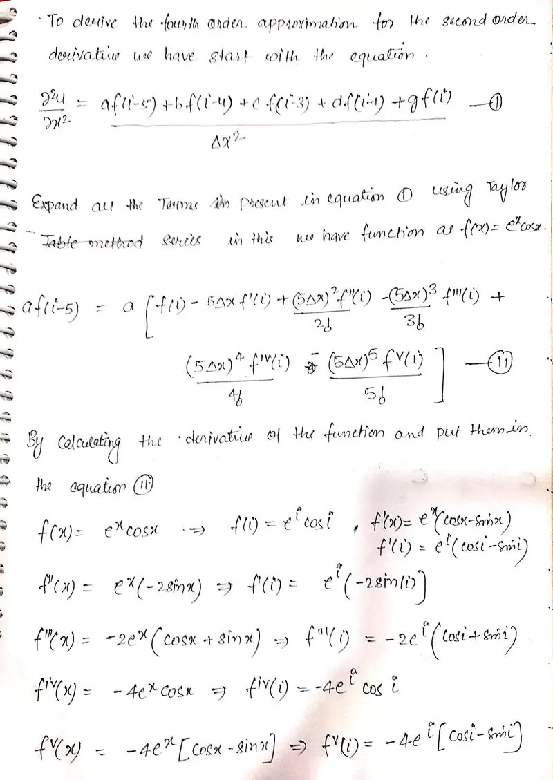
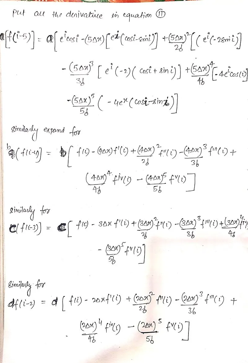
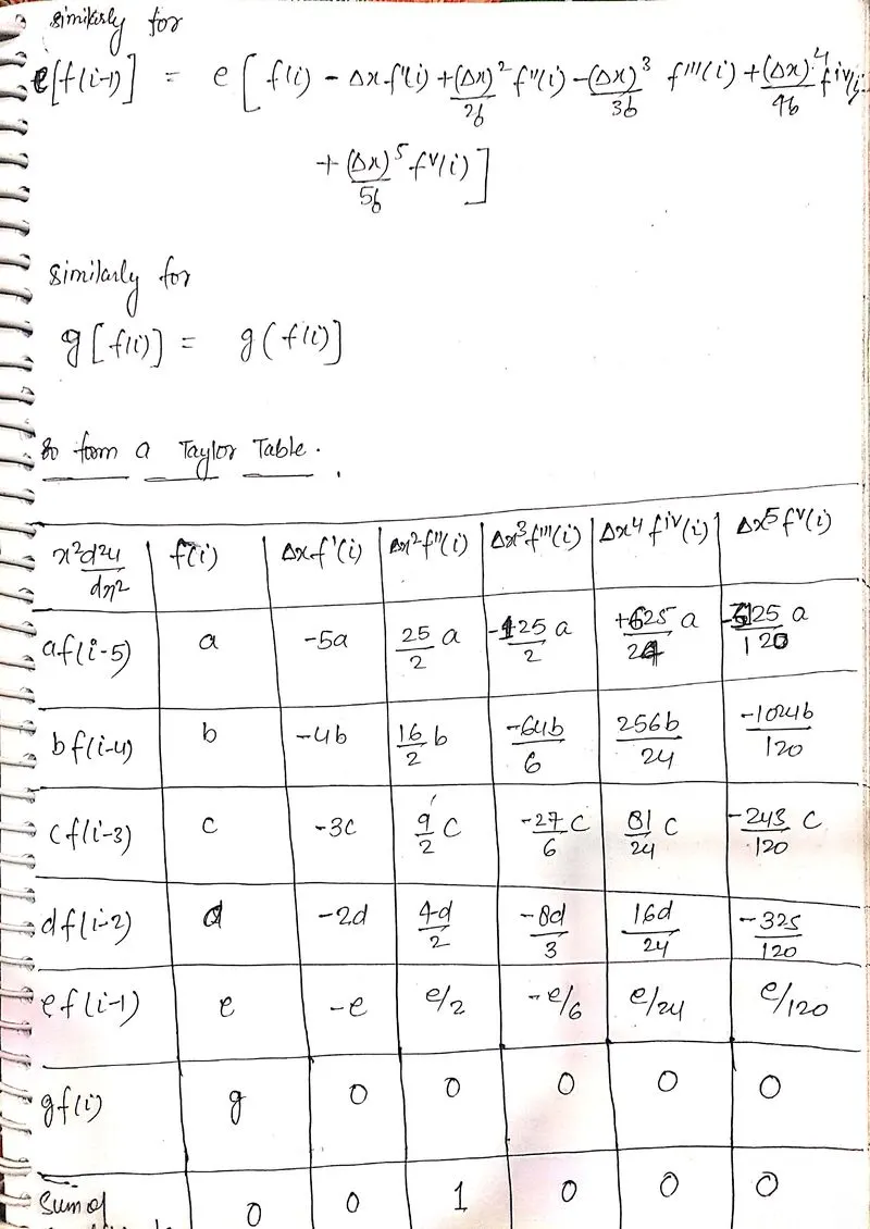
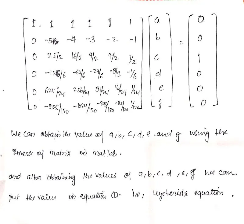
the linear equation obtained from the above table are solved using matrix inversion method
X = inv(A)*B
we get the coefficients as,so the matlab code for tthe inverse of matrix is as follows
>> format short g
>>
>> A = [1 1 1 1 1 1;0 -5 -4 -3 -2 -1;0 25/2 16/2 9/2 4/2 1/2;0 -125/6 -64/6 -27/6 -8/3 -1/6; 0 625/24 256/24 81/24 16/24 1/24;0 -3125/120 -1024/120 -243/120 -32/120 -1/120]

A =

            1            1            1            1            1            1
            0           -5           -4           -3           -2           -1
            0         12.5            8          4.5            2          0.5
            0      -20.833      -10.667         -4.5      -2.6667     -0.16667
            0       26.042       10.667        3.375      0.66667     0.041667
            0      -26.042      -8.5333       -2.025     -0.26667   -0.0083333

>> adjoint(A)

ans =

       38.333       59.194       42.694        -4.25      -32.333      -18.333
  -1.3393e-15            4       9.6667         1.75          -16          -15
   4.9181e-15      -20.417      -48.861       -10.25       66.333           55
   1.8015e-15       35.556       84.222         24.5      -70.667      -56.667
  -1.3693e-15           -5      -17.833        -29.5          -26          -10
  -3.6939e-15      -73.333      -69.889        17.75       78.667           45

>> det(A)

ans =

       38.333

>> inverse_of_A = adjoint(A)/det(A)

inverse_of_A =

            1       1.5442       1.1138     -0.11087     -0.84348     -0.47826
  -3.4939e-17      0.10435      0.25217     0.045652     -0.41739      -0.3913
    1.283e-16     -0.53261      -1.2746     -0.26739       1.7304       1.4348
   4.6997e-17      0.92754       2.1971      0.63913      -1.8435      -1.4783
   -3.572e-17     -0.13043     -0.46522     -0.76957     -0.67826     -0.26087
  -9.6362e-17       -1.913      -1.8232      0.46304       2.0522       1.1739


>> % coefficient matrix is given by the X = inverse_of_A*B
>> X = inverse_of_A*B
Error using  *
Incorrect dimensions for matrix multiplication. Check that the number of columns in the first matrix matches the number of rows in the second
matrix. To operate on each element of the matrix individually, use TIMES (.*) for elementwise multiplication.

Related documentation

>> B = [0;0;1;0;0;0]

B =

     0
     0
     1
     0
     0
     0

>>
>> % coefficient matrix is given by the X = inverse_of_A*B
>>
>> X = inverse_of_A*B

X =

       1.1138
      0.25217
      -1.2746
       2.1971
     -0.46522
      -1.8232

>> format rat
>> X

X =

    1537/1380
      29/115
    -789/619
     758/345
    -107/230
    -629/345
we get the coefficients as
a = 1537/1380, b = 29/115, c= -789/619, d =758/345, e = -107/230, g = -629/345.
hysterisis equation is given by
``(del^2u)/(delx^2) = (af(i-5) +bf(i-4)+cf(i-3)+df(i-2)+ef(i-1)+gf(i))/dx^2```
sbstituting the values in hysterisis equation
`(del^2u)/(delx^2) = (1537/1380f(i-5) +29/115f(i-4)-789/619f(i-3)+758/345f(i-2)-107/230f(i-1)-629/345f(i))/dx^2``
SKEWED RIGHT HAND DIFFERENCE SCHEME:
NO OF NODES:
The number of nodes = p+q
Where, p is order of derivative.
q is order of approximations.
The no of nodes = 2+4 =>6.
DERIVATION:
To derive a fourth order approximation for the second order derivative,we start with these approximation,
`(del^2u)/(delx^2) = (a f ( i ) + b f ( i + 1 ) + c f ( i + 2 ) + d f ( i + 3 ) + e f ( i + 4 ) + g f ( i + 5 ))/ (d x ^2)`
expand all the terms in the equation (2) using taylor series expansion and are represented in the form of table using taylor table method.
| `((del^2u)/(delx^2))dx^2` | f(i) | f'(i)dx | `(dx)^2*f''(i)` | `(dx^3)f'''(i)` | `(dx)^5f''''(i)` | `(dx)^5*f'''''(i)` |
| af(i) | a | 0 | 0 | 0 | 0 | 0 |
| bf(i+1) | b | b | b/2 | b6">b/6 | `b/24` | b120">b/120 |
| cf(i+2) | c | 2c | 4c2">4c/2 | 8c6">8c/6 | 16c24">16c/24 | 32c120">32c/120 |
| df(i+3) | d | 3d | 9d2">9d/2 | 27d6">27d/6 | 81d24">81d/24 | 243d120">243d/120 |
| ef(i+4) | e | 4e | 16e2">16e/2 | 64e6">64e/6 | 256e24">256e/24 | 1024e120">1024e/120 |
| gf(i+5) | g | 5g | 25g2">25g/2 | 125g6">125g/6 | 625g24">625g/24 | 3125g120">3125g/120 |
| sum of co_efficients | 0 | 0 | 1 | 0 | 0 | 0 |
the linear equation obtained from the above table are solved using matrix inversion method,
A.X = B
the coefficients will be solved using the matrix inversion method using matlab.
matlab code for the matrix inversion is shown below
>> format short g
>>
>> A = [1 1 1 1 1 1;0 1 2 3 4 5;0 1/2 4/2 9/2 16/2 25/2;0 1/6 8/6 27/6 64/6 125/6;0 1/24 16/24 81/24 256/24 625/24;0 1/120 32/120 243/120 1024/120 3125/120]

A =

            1            1            1            1            1            1
            0            1            2            3            4            5
            0          0.5            2          4.5            8         12.5
            0      0.16667       1.3333          4.5       10.667       20.833
            0     0.041667      0.66667        3.375       10.667       26.042
            0    0.0083333      0.26667        2.025       8.5333       26.042

>> adjoint(A)

ans =

            1      -2.2833         3.75        -4.25            3           -1
   -2.823e-17            5      -12.833        17.75          -14            5
  -1.3241e-16           -5       17.833        -29.5           26          -10
  -2.8537e-17       3.3333          -13         24.5          -24           10
   4.6092e-17        -1.25       5.0833       -10.25           11           -5
  -8.7603e-17          0.2     -0.83333         1.75           -2            1

>> det(A)

ans =

            1

>> inverse_of_A = adjoint(A)/det(A)

inverse_of_A =

            1      -2.2833         3.75        -4.25            3           -1
   -2.823e-17            5      -12.833        17.75          -14            5
  -1.3241e-16           -5       17.833        -29.5           26          -10
  -2.8537e-17       3.3333          -13         24.5          -24           10
   4.6092e-17        -1.25       5.0833       -10.25           11           -5
  -8.7603e-17          0.2     -0.83333         1.75           -2            1

>> % solution matrix is given by B
>> B = [0;0;1;0;0;0]

B =

     0
     0
     1
     0
     0
     0

>> %coefficient matrix is given by X
>>
>> X = inverse_of_A*B

X =

         3.75
      -12.833
       17.833
          -13
       5.0833
     -0.83333

>> format rat
>> X

X =

      15/4
     -77/6
     107/6
     -13
      61/12
      -5/6
so the value of coefficients are
a = 15/4; b =-77/6; c = 107/6 ; d= -13; e = 61/12; g = -5/6;
put the value of coefficients in the hysterisis equation
`(del^2u)/(delx^2) = (15/4 f ( i ) -77/6 f ( i + 1 ) + 107/6 f ( i + 2 ) -13 f ( i + 3 ) + 61/12 f ( i + 4 ) -5/6 f ( i + 5 ))/ (d x ^2)``
# matlab code;
clear all
close all
clc

x = pi/3;
dx = linspace(pi/40,pi/4,10);

for i =1:length(dx)

    central_diifrence_approximation_error(i) = cdsa(x,dx(i))

    skewed_Right_sided_approximation_error(i)= srsa(x,dx(i))

    skewed_left_sided_approximation_error(i) = slsa(x,dx(i))

end

%plotting

figure(1)
loglog(dx,central_diifrence_approximation_error,'color','r')
hold on
loglog(dx,skewed_Right_sided_approximation_error,'color','b')
hold on

loglog(dx,skewed_left_sided_approximation_error)

xlabel('dx')

ylabel('fourth_order_approximation_error_for_second_order_derivative')

legend('central_diffrence_approximation_error','skewed_right_sided_approximation_error','skewed_left_sided_approximation_error')
# function for the central_diffrence_approximation_error;
function[output] = cdsa(x,dx)

%analytical second order derivative

analytical_second_order_derivative = -2*sin(x)*exp(x);

% central_scheme_second_order_derivative

central_scheme_second_order_derivative =  ((7/12)*(exp(x-(2*dx))*cos(x-(2*dx)) -4*(exp(x-dx)*cos(x-dx)) -(5/12)*(exp(x)*cos(x)) +(20/3)*(exp(x+dx)*cos(x+dx)) -(3/4)*(exp(x+(2*dx))*cos(x+(2*dx))))/(dx)^2);


output = abs(analytical_second_order_derivative - central_scheme_second_order_derivative);

end
# fuction for the skewed right sided approximation error
function[output] = srsa(x,dx)

%analytical second order derivative

analytical_second_order_derivative = -2*sin(x)*exp(x);

skewed_right_sided_numerical_approximation =  ((15/4)*(exp(x)*cos(x))) -((77/6)*(exp(x+dx)*cos(x+dx)))+((107/6)*(exp(x+(2*dx))*cos(x+(2*dx)))) -(13*(exp(x+(3*dx))*cos(x+(3*dx)))) + (61/12*(exp(x+(4*dx))*cos(x+(4*dx)))) -(5/6)*(exp(x+(5*dx))*cos(x+(5*dx)))/(dx)^2;

output = abs(analytical_second_order_derivative-skewed_right_sided_numerical_approximation);

end
# function for skewed left sided approximation error
function[output] = slsa(x,dx)

%analytical second order derivative

analytical_second_order_derivative = -2*sin(x)*exp(x);

% skewed_left_sided_numerical_approximation

skewed_left_sided_numerical_approximation = ((1537/1380)*(exp(x-5*dx)*cos(x-5*dx)))+(29/115*(exp(x-4*dx)*cos(x-4*dx)))-((789/619)*(cos(x-3*dx)*exp(x-3*dx)))+(758/345*(exp(x-2*dx)*cos(x-2*dx)))-(107/230*(exp(x-dx)*cos(x-dx))-629/345*(exp(x)*cos(x)))/(dx)^2;

% error

output = abs(analytical_second_order_derivative-skewed_left_sided_numerical_approximation);

end
#output;
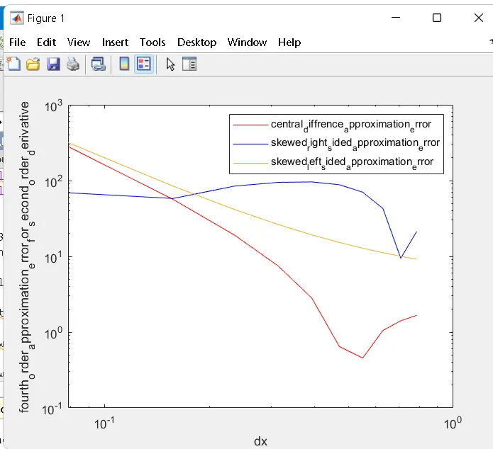
central_diifrence_approximation_error =

  281.1815   56.4805   19.1102    7.5041    2.8201    0.6458    0.4548    1.0533    1.4119    1.6661


skewed_Right_sided_approximation_error =

   69.0533   58.0994   84.5430   94.7614   96.0332   88.1904   70.3052   42.8474    9.4379   21.3093


skewed_left_sided_approximation_error =

  317.0110   84.5650   41.5770   26.3805   19.2249   15.2607   12.8186   11.1907   10.0329    9.1627
plot for the diffrent types of error;
conclusion;
> As the value of dx increases the value of the error will also increases in all three cases which is what we expecting because at the higher value of dx the larger value will be neglected due to which the error will also increases.
> As seen from the plot, the central differencing scheme has very less error compared to other schemes. Therefore, central differencing is better than other schemes because it uses information from both the sides from the point of consideration to give approximative and accurate values.
As the left and right skewed difference methods uses data only from one side of point of interest it gives less approximative and accurate values about the point.