Week 3.5 - Deriving 4th order approximation of a 2nd order derivative using Taylor Table method

close all
clear all
clc

x = pi/30;
dx = linspace(pi/30, pi/300, 10);

for i = 1:length(dx)

    CD_error(i) = Centrl_difrncing(x,dx(i));
    Skew_RHS_error(i) = Skew_RHS(x,dx(i));
    Skew_LHS_error(i) = Skew_LHS(x,dx(i));

end

figure(1)
loglog(dx,CD_error,'r')
hold on
loglog(dx, Skew_RHS_error,'b')
hold on
loglog(dx, Skew_LHS_error,'g')
xlabel('dx_Step size')
ylabel('Error aproximation')







 
function out_1 = Centrl_difrncing(x,dx)


f_x = exp(x)*cos(x);

Analytical_derrivative = -2*exp(x)*sin(x)


A= [1 -2 2 -4/3 2/3; 1 -1 0.5 -1/6 1/24; 1 0 0 0 0; 1 1 0.5 1/6 1/24; 1 2 2 4/3 2/3];

B = [0 0 1 0 0];

Z = B*inv(A);

a = Z(1);
b = Z(2);
c = Z(3);
d = Z(4);
e = Z(5);


Central_diff = (a*((exp(x-(2*dx))*cos(x-(2*dx))))  +  b*((exp(x-dx)*cos(x-dx)))  +  c*(exp(x)*cos(x))  +  d*((exp(x+dx)*cos(x+dx)))  +  e*((exp(x+(2*dx))*cos(x+(2*dx)))))  /  (2*dx^2);

out_1 = abs(Analytical_derrivative - Central_diff)



end





 
function out_2 = Skew_RHS(x,dx)

f_x = exp(x)*cos(x);

Analytical_derrivative = -2*exp(x)*sin(x);

C = [1 0 0 0 0; 1 1 0.5 0.5 1/6; 1 2 2 8/6 16/24; 1 3 4.5 27/6 81/24; 1 4 8 64/6 256/24];

D = [0 0 1 0 0];

ZZ = D*inv(C);

aa = ZZ(1);
bb = ZZ(2);
cc = ZZ(3);
dd = ZZ(4);
ee = ZZ(5);

Skew_RH = (aa*(exp(x)*cos(x))  +  bb*((exp(x+dx)*cos(x+dx)))  +  cc*((exp(x+(2*dx))*cos(x+(2*dx))))  +  dd*((exp(x+(3*dx))*cos(x+(3*dx))))  +  ee*((exp(x+(4*dx))*cos(x+(4*dx)))));

out_2 = abs(Analytical_derrivative - Skew_RH)

end


 
function out_3 = Skew_LHS(x,dx)


f_x = exp(x)*cos(x);

Analytical_derrivative = -2*exp(x)*sin(x);

E = [1 -5 25/2 -125/6 625/24; 1 -4 8 -64/6 256/24; 1 -3 4.5 -27/6 81/24; 1 -2 2 -8/6 16/24; 1 -1 0.5 -1/6 1/24];

F = [0 0 1 0 0];
ZZZ = F*inv(E);

aaa = ZZZ(1);
bbb = ZZZ(2);
ccc = ZZZ(3);
ddd = ZZZ(4);
eee = ZZZ(5);

Skew_LH =  (aaa*((exp(x-(4*dx))*cos(x-(4*dx))))  +  bbb*((exp(x-(3*dx))*cos(x-(3*dx))))  +  ccc*((exp(x-(2*dx))*cos(x-(2*dx))))  +  ddd*((exp(x-dx)*cos(x-dx)))  +  eee*(exp(x)*cos(x)));

out_3 = abs(Analytical_derrivative - Skew_LH)


end

 
 


CONCLUSION:
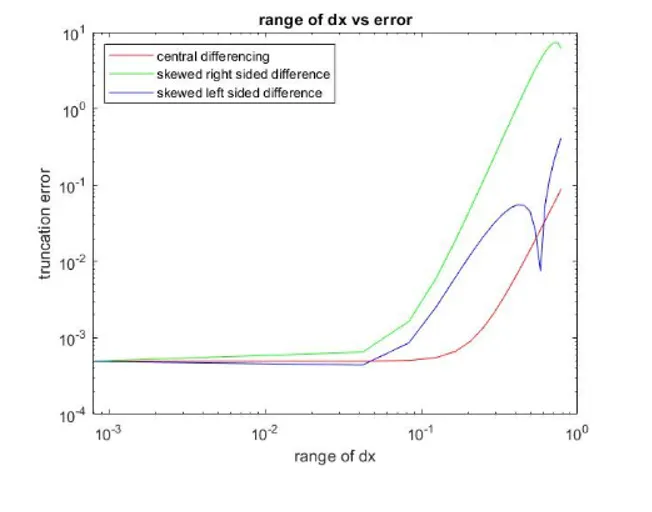
               As seen from the plot, the central differencing scheme has very less error compared to other schemes. Therefore, central differencing is better than other schemes because it uses information from both the sides from the point of consideration to give approximative and accurate values.
               As the left and right skewed difference methods uses data only from one side of point of interest it gives less approximative and accurate values about the point.