Week 3.5 - Deriving 4th order approximation of a 2nd order derivative using Taylor Table method

Aim :- To derive 4th order approximation of a 2nd order derivative using Taylor Table method and need to plot the error for the diffrent schemes against the range of dx

Steps : -

• First we have to derive the hypothesis equation for the central diffrence , Skewed right-sided difference and skewed left-sided difference of 4 th order approximation of second order derivative
• Then using Taylor table method we need to find the coefficient of the talor table terms by expanding the derivative terms of the hypothesis equation using taylor series expansion
• After using MATLAB 'linsolve' inbuilt command (AX = B , syntax= 'X =linsolve(A,B)') programming we can calculate the unknown coefficient (a,b,c,d,e,g) [For central difference schemes we have 5 unknown coefficients]
• We have to write the MATLAB programming in order to calculate the errors for the given range of dx and plot the error against the range of dx

Scheme Derivations:

Central Difference Scheme :

No of nodes = p+q-1 ,[where p = order of derivatives, q = order of approximation]

= 2+4-1

= 5

Hyptothesis equation of the central difference scheme of a second order derivative

`(d^2u)/(dx^2 )=(af(i-2)+bf(i-1)+cf(i)+df(i+1)+ef(i+2))/(∆x^2 )`

Taylor series expansion of the first term of the equation :

`af(i-2) = a(f(i)-((2dx)f'(i))/(1)+((2dx)^2f''(i))/(2!)-((2dx)^3f'''(i))/(3!)+((2dx)^4f''''(i))/(4!)-((2dx)^5f'''''(i))/(5!)+......)`

Similarly by expanding all the terms in terms of taylor series expansion , taylor table has formed.

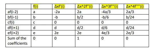
Sum of the coefficients of the first order derivatives, `1+1+1+1+1 = 0 rarr (1)`

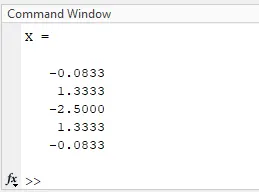
In this similar way we have written down all the 5 eqautions and then calculated the coefficients (a,b,c,d,e) in MATLAB programming.

Skewed right-sided difference :

No of nodes = p+q ,[where p = order of derivatives, q = order of approximation]

= 2+4

= 6

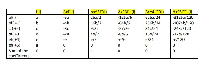
Hyptothesis equation of Skewed right-sided difference scheme of a second order derivative :

`(d^2u)/(dx^2 )=(af(i)+bf(i+1)+cf(i+2)+df(i+3)+e(i+4)+gf(i+5))/(∆x^2 )`

Taylor table :

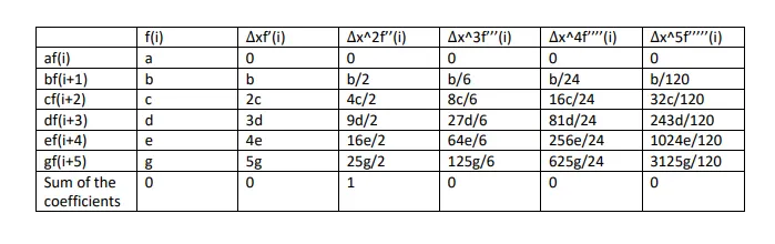
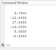
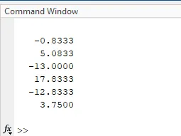
We have caiculated the coefficients in MATLAB as you can see in the below pic of command window

Skewed left-sided difference scheme :

No of nodes = p+q ,[where p = order of derivatives, q = order of approximation]

= 2+4

= 6

Hyptothesis equation of Skewed left-sided difference scheme of a second order derivative :

`(d^2u)/(dx^2 )=(af(i)+bf(i-1)+cf(i-2)+df(i-3)+e(i-4)+gf(i-5))/(∆x^2 )`

Taylor table :

Coefficients (a,b,c,d,e,g)

MATLAB CODE TO CALCULATE THE ERRORS AND FOR PLOTTING

Main Code

% Fourth order approximation of second order derivative
clear all % To clear all existing variables in workspace 
close all % Closed figure window
clc % In order to clear command window

%value of x
x= pi/3;

% To create an array  of dx
dx= linspace(pi/4,pi/4000,20);

%for loop to execute a same  action for the requires times
for i=1:length(dx)
    
    central_differencing_error(i) = cdo_order(x,dx(i));
    
    right_sided_skew_error(i) = rsk(x,dx(i));
    
    left_sided_skew_error(i) = lsk(x,dx(i));
    
end

%plotting using loglog command 
figure(1)
loglog(dx,central_differencing_error,'b--o')
hold on
loglog(dx,right_sided_skew_error,'r--o')
loglog(dx,left_sided_skew_error,'k--o')
xlabel('dx')
ylabel('truncation error')
title('range of dx vs error')
legend('central differencing','skewed right sided difference','skewed left sided difference','location','northwest')

%plotting using plot command 
figure(2)
plot(dx,central_differencing_error,'b--o')
hold on
plot(dx,right_sided_skew_error,'r--o')
plot(dx,left_sided_skew_error,'k--o')
xlabel('dx')
ylabel('truncation error')
title('range of dx vs error')
legend('central differencing','skewed right sided difference','skewed left sided difference','location','northwest')

Function code for central difference scheme

function Error_central_differencing =cdo_order(x,dx)

%  AX = B to calculate the coefficients 
a3 = [1 1 1 1 1 ; -2 -1 0 1 2 ; 2 0.5 0 0.5 2 ; -4/3 -1/6 0 1/6 4/3 ; 2/3 1/24 0 1/24 2/3 ];
b3=[0 ;0;1;0;0;];
c = linsolve(a3,b3);
% analytic function = exp(x)*cos(x)

% analytic derivative
%f''(x) = -2*exp(x)*sin(x)

analytical_derivative = -2*exp(x)*sin(x);

%numerical derivative

% Central diffrencing 
f = @ (x) exp(x)*cos(x);
central_differencing = (c(1)*f(x-(2*dx))+c(2)*f(x-(1*dx))+c(3)*f(x)+c(4)*f(x+(1*dx))+c(5)*f(x+(2*dx)))/dx^2;

%error
Error_central_differencing = abs(central_differencing- analytical_derivative);
end

Function code for Skewed right-sided difference scheme

function Error_right_sided_skew = rsk(x,dx)

%  AX = B to calculate the coefficients 
a3 = [1 1 1 1 1 1 ; 0 1 2 3 4 5 ; 0 1/2 2 4.5 8 12.5 ; 0 1/6 8/6 27/6 64/6 125/6 ; 0 1/24 16/24 81/24 256/24 625/24 ; 0 1/120 32/120 243/120 1024/120 3125/120 ];
b3=[0 ;0;1;0;0;0];
c = linsolve(a3,b3);
% analytic function = exp(x)*cos(x)

% analytic derivative
%f''(x) = -2*exp(x)*sin(x)

analytical_derivative = -2*exp(x)*sin(x);

%numerical derivative

%central differencing
f = @ (x) exp(x)*cos(x);
right_sided_skew =(c(1)*f(x)+c(2)*f(x+(1*dx))+c(3)*f(x+(2*dx))+c(4)*f(x+(3*dx))+c(5)*f(x+(4*dx))+c(6)*f(x+(5*dx)))/dx^2;

%error
Error_right_sided_skew = abs(right_sided_skew- analytical_derivative);
end

Function code for skewed left-sided difference scheme

function Error_left_sided_skew = lsk(x,dx)

%  AX = B to calculate the coefficients 
a3=[1  1 1 1 1 1 ; 0 -1 -2 -3 -4 -5 ; 0, 1/2,  4/2,  9/2, 16/2, 25/2; 0, -1/6, -8/6, -27/6, -64/6, -125/6; 0, 1/24, 16/24, 81/24, 256/24, 625/24;  0, -1/120, -32/120, -243/120, -1024/120, -3125/120];
b3=[0 ;0;1;0;0;0];
c = linsolve(a3,b3);
% analytic function = exp(x)*cos(x)

% analytic derivative
%f''(x) = -2*exp(x)*sin(x)

analytical_derivative = -2*exp(x)*sin(x);

%numerical derivative
f = @ (x) exp(x)*cos(x);
left_sided_skew = (c(1)*f(x)+c(2)*f(x-(1*dx))+c(3)*f(x-(2*dx))+c(4)*f(x-(3*dx))+c(5)*f(x-(4*dx))+c(6)*f(x-(5*dx)))/dx^2;

%error
Error_left_sided_skew = abs(left_sided_skew- analytical_derivative);
end

Explanation of the code :

• First of all as usual close all,clear all and clc has been used in order to clear all the existing variables in workspace, figure windows and command window respectively.
• Then given the input and created an array of dx using linspace command to see the doffrence in error with the decreasing of dx value.
• We have written three function code for the three different schemes where I have calculated the coefficients and the errors by substituting the analytical derivatives from skew schemes .
• And for simplifying the equation inline function syntax : 'f = @ (x) x ' has been used .
• Then in the main script file we have called the functions code and then plotted the error aginst the range of dx using two difference inbuilt command loglog and plot.

Output:-

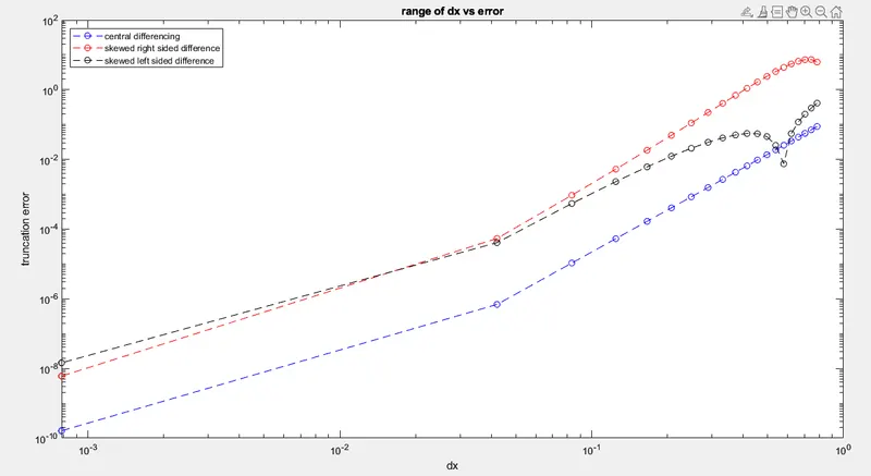
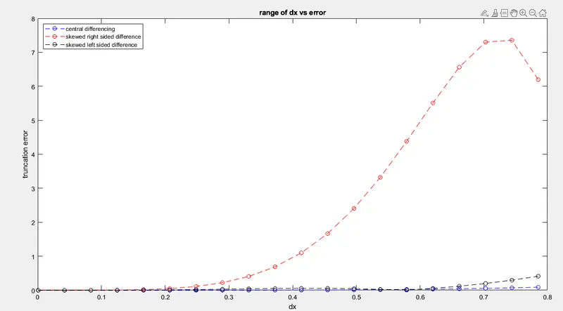
Graph Error vs Range of dx

Using loglog command

Using plot command

Conclusions :-

By observing the above plots it is cleared that , the central differencing scheme has very less error compared to other two schemes. So, central differencing is better than compared to other two schemes because it takes information from both sides of the initial point to give most accurate result. And also right-sided scheme gives less error compare to left-sided schemes.

As the left and right skewed difference methods uses data only from one side of point of interest it gives less approximative and accurate values about the point.

Why a skewed scheme is useful compare to FDS and BDS ?

At forwords and backward difference schemes we can calculate error at boundary , but it wont be good decision because FDS and BDS has low order of approximation so it would be have more error. Therefore,skewed difference scheme is prefer for such case.

What can a skewed scheme do that a cd scheme cannot do :

CDS cannot not be employed at the boundary nodes due to unavailability of right and left nodes at the same time. In such cases the skewed differencing scheme is used.