Week 3.5 - Deriving 4th order approximation of a 2nd order derivative using Taylor Table method

Aim - Deriving the 4th order approximations of the second-order derivative.

Objective -

1. Central difference

2. Skewed right-sided difference

3. Skewed left-sided difference

4. describe why a skewed scheme is useful? What can a skewed scheme do that a CD scheme cannot?

Theory -

Taylor Series - An infinite sum of terms that are expressed in terms of the function's derivatives at a single point. For most common functions, the function and the sum of its Taylor series are equal near this point.

The order of accuracy for the central difference method can be found as:

P = N - Q + 1

Where,

P is The order of accuracy

N is the number of nodes in the stencil

Q is the order of derivative

Therefore the number of nodes to be considered for a fourth-order accurate approximation of a second-order derivative by central difference method is given by:

4 = N -2+1

N = 5.

1) Skewed 2nd order right-sided difference scheme

The number of Nodes required for 4th order approximation of a second-order derivative can be given by the equation

N=P+Q

`Q(d^2y)/dx^2 = (af(i)+bf(i+1)+cf(i+2)+df(i+3)+ef(i+4)+gf(i+5))/(Delta x^2)`

P af(i) = af(i) is the order of approximation

So, here we need 6 nodes in order to find the 2nd order derivative with the 4th order of approximation.

2) Skewed 2nd order Left-sided difference scheme

The number of Nodes required for 4th order approximation of a second-order derivative can be given by the equation

N=P+Q

So, here we need 6 nodes in order to find the 2nd order derivative with the 4th order of approximation.

`(d^2y)/dx^2`

3) Symmetric central difference scheme

The number of Nodes required for 4th order approximation of a second-order derivative can be given by the equation

N=P+Q

So, here we need 5 nodes in order to find the 2nd order derivative with the 4th order of approximation.

`(d^2y)/dx^2 = (af(i-2)+bf(i-1)+cf(i)+df(i+1)+ef(i+2)) / (Delta x^2)`

Program Codes -

% Deriving 4th order approximation
% Using Taylor Table method

clear
close 
clc
  
%inputs
  
x = pi/3;

dx = linspace(pi/4,pi/400,500);    % Stepsize range
  
% Analytical derivative
  
% f(x) = exp(x)*cos(x)
% f'(x)=(exp(x)*cos(x)-(exp(x)*sin(x)=exp(x)*(cosx-sinx)
% Double derivative f" = -2*exp(x)*sin(x)
  
analytical_derivative = -2*exp(x)*sin(x);
  
% Skewed Right-sided(4th order approimation)
% Solving for the coefficients
A = [1 1 1 1 1 1;0 1 2 3 4 5;0 1/2 4/2 9/2 16/2 25/2;0 1/6 8/6 27/6 64/6 125/6;0 1/24 16/24 81/24 256/24 625/24;0 1/120 32/120 243/120 1024/120 3125/120];
B = [0;0;1;0;0;0];
x_right = inv(A)*B;
  
% Skewed Left-sided(4th order approimation)
% Solving for the coefficients
C = [1 1 1 1 1 1;0 -1 -2 -3 -4 -5;0 1/2 4/2 9/2 16/2 25/2;0 -1/6 -8/6 -27/6 -64/6 -125/6;0 1/24 16/24 81/24 256/24 625/24;0 -1/120 -32/120 -243/120 -1024/120 -3125/120];
D = [0;0;1;0;0;0];
x_left = inv(C)*D;
  
% Central differencing(4th order approimation)
% Solving for the coefficients
E = [1, 1, 1, 1, 1;-2, -1, 0, 1, 2;4/2, 1/2, 0, 1/2, 4/2;-8/6, -1/6, 0, 1/6, 8/6;16/24, 1/24, 0, 1/24, 16/24];
F = [0;0;1;0;0];
x_central = E^-1*F;

% Anonymous Function
  
f=@(x) exp(x).*cos(x);
  
  
% Numerical derivative
  
right_difference = (x_right(1)*f(x)+x_right(2)*f(x+dx)+x_right(3)*f(x+2.*dx)+x_right(4)*f(x+3.*dx)+x_right(5)*f(x+4.*dx)+x_right(6)*f(x+5.*dx))./(dx.^2);
 
left_difference = (x_left(1)*f(x)+x_left(2)*f(x-dx)+x_left(3)*f(x-2.*dx)+x_left(4)*f(x-3.*dx)+x_left(5)*f(x-4.*dx)+x_left(6)*f(x-5.*dx))./(dx.^2); 

cent_difference = (x_central(1)*f(x-2.*dx)+x_central(2)*f(x-1.*dx)+x_central(3)*f(x)+x_central(4)*f(x+dx)+x_central(5)*f(x+2.*dx))./(dx.^2);

% Absolute error
  
error_r = abs(analytical_derivative-right_difference);
error_l = abs(analytical_derivative-left_difference);
error_c = abs(analytical_derivative-cent_difference);
error = [error_r;error_l;error_c];
  
% Plotting loglog graph

figure(1)
loglog(dx,error_r) 
hold on
loglog(dx,error_l)
loglog(dx,error_c)
xlabel('Range of dx')
ylabel('Absolute Error')
legend('Right Differencing','Left Differencing','Central Differencing')
     
  

Code Explanation:

Step1: clear all – command to clear the workspace.

Step 2: close all – command to close all opened previous plots.

Step 3: clc – command to clear the command window.

Step 4: Define the input value of 'x =pi/3' to be solved for the function.

Step 5: defining the discretization range as array 'dx =(pi/4,pi/400,500)'.

Step 6: computing the numerical approximation error value of the second derivative of the given function by calling a function code.

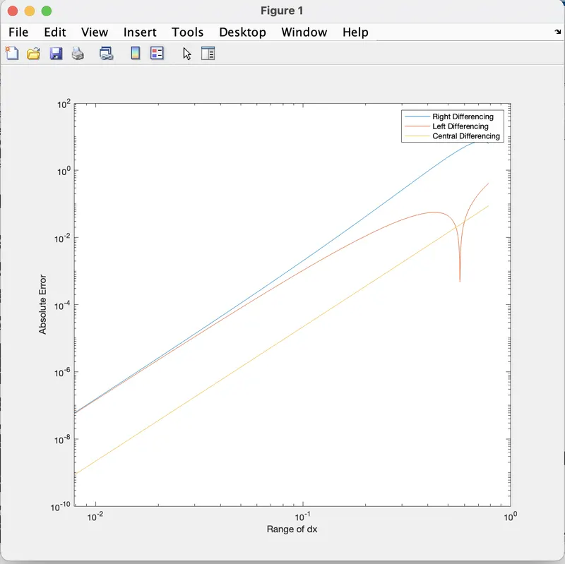
Output Graph -

Explaination -

As we can see from the above figure the error for the central difference method is very less compared to the skewed methods.

Skewed right and left difference methods almost gives the same results in terms of error for a small value of time step.

• When data from the grid points is only available from either the left or right end i.e. at nodes closer to the boundaries,for computations that requires a high order approximations we make use of skewed schemes.Having a symmetric stencil for computation is not possioble in this scenarios like we do for central differencing schemes or having a low order accuracy.For better consistency of scheme to be maintained the values of dx are kept as low as possible for providing proper computational plots.
• A skewed scheme is useful when we have to predict using the boundary condition as we have only one direction to go. Hence the skewed scheme will be useful and we cannot use the central differencing scheme for such an application because it required information from both directions of the point.

Why a skewed scheme is useful?

The system which doesn’t contain sufficient information on both side of the point of interest. In such cases we cannot use central differencing scheme so skewed scheme is useful in such cases.

What can a skewed scheme do that a CD scheme cannot do?

Since we can see that the central differencing scheme gives us more immaculate solutions or lesser errors as compared to the skewed difference scheme. But it is not always viable to use the central differencing to evaluate solutions. Suppose, if we want to compute numerical approximations for a function at the boundary or corner node; we cannot use the central difference scheme at this particular situation because it requires data from both sides of the node or boundary. So, in this situation skewed difference method plays a major role; as in the skewed scheme data from one side can be used to compute numerical approximation at a point.

Conclusion -

Successfully plotted a graph for Deriving the 4th order approximations of the second-order derivative, in which the central differencing scheme has very less error compared to other schemes. Therefore, central differencing is better than other schemes because it uses information from both the sides from the point of consideration to give approximative and accurate values.

As the left and right skewed difference methods uses data only from one side of point of interest it gives less approximative and accurate values about the point.