Week 3.5 - Deriving 4th order approximation of a 2nd order derivative using Taylor Table method

clear all 
close all
clc
%x value
x=pi/4;
%dx value equaly devided into 10 from pi/3 to pi/30
dx=linspace(pi/3,pi/30,10);
%berfore solving using numerical method first calculate for analatucal
%method 
analytical=-2*exp(x)*sin(x);
% A1,B1 is defined form taylor table
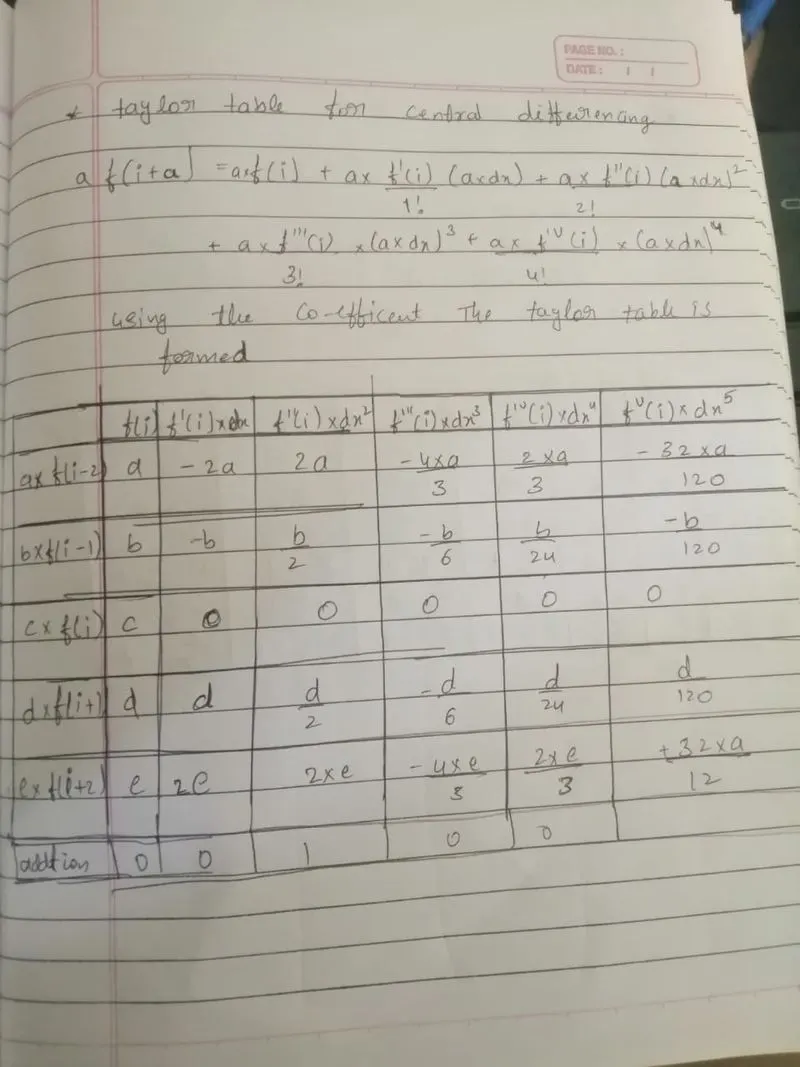
A1=[1 1 1 1 1 ;-2 -1 0 1 2;2 1/2 0 1/2 2;-4/3 -1/6 0 1/6 4/3;2/3 1/24 0 1/24 2/3];
B1=[0;0;1;0;0];
%x is sovlved using matrix properties

X1=inv(A1)*B1;
a1=X1(1);
b1=X1(2);
c1=X1(3);
d1=X1(4);
e1=X1(5);
% A2,B2 is defined form taylor table for right skewed difference
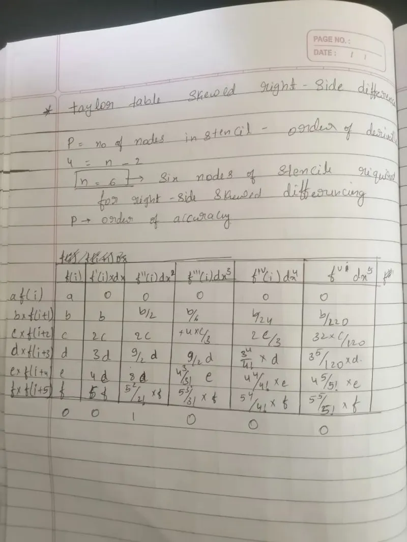
A2=[1 1 1 1 1 1;0 1 2 3 4 5;0 1/2 2 9/2 8 (5^2/2);0 1/6 4/3 9/2 (4^3/6) (5^3/6);0 1/24 2/3 (3^4/24) (4^4/24) (5^4/24);0 1/120 32/120 3^5/120 4^5/120 5^5/120];
B2=[0;0;1;0;0;0];
X2=inv(A2)*B2;
a2=X2(1);
b2=X2(2);
c2=X2(3);
d2=X2(4);
e2=X2(5);
f2=X2(6);
% A3,B3 is defined form taylor table for left skewed difference
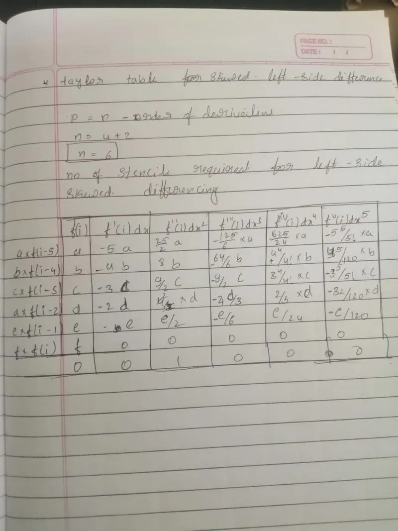
A3=[1 1 1 1 1 1;-5 -4 -3 -2 -1 0; 25/2 8 9/2 2 1/2 0;-125/6 -64/6 -9/2 -4/3 -1/6 0;625/24 4^4/24 3^4/24 2/3 1/24 0;-5^5/120 -4^5/120 -3^5/120 -32/120 -1/120 0];
B3=[0;0;1;0;0;0];
X3=inv(A3)*B3;
a3=X3(1);
b3=X3(2);
c3=X3(3);
d3=X3(4);
e3=X3(5);
f3=X3(6);
%to solve approximaton for all dx value and their error using for loop
for i=1:length(dx)
    %for center difference 
term1_1=a1.*(exp(x-2.*dx(i)).*cos(x-2.*dx(i)));
term2_1=b1.*(exp(x-dx(i)).*cos(x-dx(i)));
term3_1=c1.*(exp(x).*cos(x));
term4_1=d1.*(exp(x+dx(i)).*cos(x+dx(i)));
term5_1=e1.*(exp(x+2.*dx(i)).*cos(x+2.*dx(i)));
%for right skewd dfference 
term1_2=a2*(exp(x)*cos(x));
term2_2=b2*(exp(x+dx(i))*cos(x+dx(i)));
term3_2=c2*(exp(x+2*dx(i))*cos(x+2*dx(i)));
term4_2=d2*(exp(x+3*dx(i))*cos(x+3*dx(i)));
term5_2=e2*(exp(x+4*dx(i))*cos(x+4*dx(i)));
term6_2=f2*(exp(x+5*dx(i))*cos(x+5*dx(i)));
%for left skewed difference 
term1_3=a3*(exp(x)*cos(x));
term2_3=b3*(exp(x+dx(i))*cos(x+dx(i)));
term3_3=c3*(exp(x+2*dx(i))*cos(x+2*dx(i)));
term4_3=d3*(exp(x+3*dx(i))*cos(x+3*dx(i)));
term5_3=e3*(exp(x+4*dx(i))*cos(x+4*dx(i)));
term6_3=f3*(exp(x+5*dx(i))*cos(x+5*dx(i)));


%approximation for center difference 
center_difference(i) = (term1_1+term2_1+term3_1+term4_1+term5_1)/(dx(i).^2);

%approximation for right skewed difference 
rigth_skewed(i) = (term1_2+term2_2+term3_2+term4_2+term5_2+term6_2)/(dx(i)^2);

%approximation for left skewed difference 
left_skewed(i)  = (term1_3+term2_3+term3_3+term4_3+term5_3+term6_3)/(dx(i).^2);


error_1=abs(center_difference-analytical);

error_2=abs(rigth_skewed-analytical);

error_3=abs(left_skewed-analytical);
end
%plots for error b/w analytical method to the numerirical approximation 
figure(1)
plot(dx,error_1)
hold on
plot(dx,error_2,'r')
plot(dx,error_3,'k')
hold off
xlabel('dx')
ylabel('error')
title('dx vs error')
legend('center difference','right skewed','left skewd')

%plots for for error bu in log scale

figure(2)
loglog(dx,error_1)
hold on
loglog(dx,error_2,'r')
loglog(dx,error_3,'k')
hold off
xlabel('log(dx)')
ylabel('log(error)')
title('logerthmic comparision dx vs error')
legend('center difference','right skewed','left skewd')

%plots for approximation 
figure(3)
plot(dx,center_difference)
hold on
plot(dx,rigth_skewed,'r')
plot(dx,left_skewed,'k')
hold off
xlabel('dx')
ylabel('approximation')
title('dx vs approximation')
legend('center difference','right skewed','left skewd')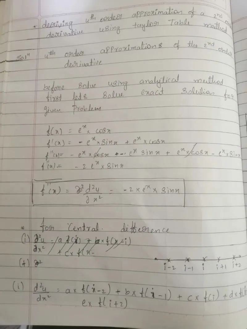

aim:-
1.derive he fouth order difference for 2nd order derivative using taylor table method
2.calculate center,skkewed right-side amd skewed left side difference
3.code he above problem using matlab and plot the result

Governing eqn :-
1.analytical soluction for f(x)=(e^(x))*cos(x) for 2nd order derivative is
f''(x)=-2*(e^(x))*sin(x)
2.for numarical maethod
A.center differnce method
to calculate no of stncile
p=n-Q+1
here p-The order of accuracy=4
n-Number of nodes in the stencil
Q-order of derivative=2
n=5

f''(x)=(a*f(x-2)+b*f(x-1)+c*f(x)+d*f(x+1)+e*f(x+2))/dx^2;

B.for skewed right side difference

p=n-Q
f''(x)=(a*f(x)+b*f(x+1)+c*f(x+2)+d*f(x+3)+e*f(x+4)+f*f(x+5)/dx^2;

C.for skewed left side difference
p=n-Q
f''(x)=(a*f(x-5)+b*f(x-4)+c*f(x-3)+d*f(x-2)+e*f(x-1)+f*f(x))/dx^2;

Body of content:-
from taylor tabel A and B is calculated using matrix property X is found which is nothing but coeefient of the our hypothesis eqn
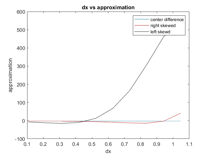
the found coeffienets is used to calculete the approximmation using hypothesis eqn
to calculate dx is diveded in equally usimg linspace command
then the used in for loop to calculate the approximation and the error associated with approximation comapered to the analyatical value
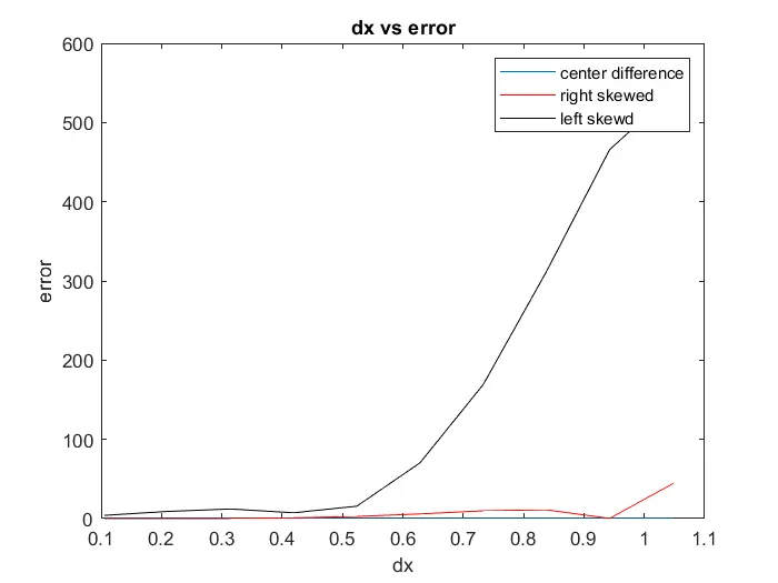
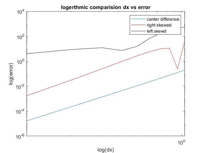
the found value like error and approxiamated value is plote d]

conclusion:-
from the plots it can be seen that for center differnce the value is found to be fore accurate compred to the othere to difference
from loglog plot also show that the center differnce gives near approximated value