Week 3.5 - Deriving 4th order approximation of a 2nd order derivative using Taylor Table method

AIM:

To derive the 4th order approximation for second-order derivative for the following

1. Central difference

2. Skewed right-sided difference

3. Skewed left-sided difference

And to prove that skewed schemes are fourth-order accurate using thumb rule(i.e 1.The order of accuracy P = Number of nodes in the stencil N - order of derivative Q + 1 for symmetric/central schemes. 2.The order of accuracy P = Number of nodes in the stencil N - order of derivative Q for one-sided/skewed schemes)

And to write a program in Matlab to evaluate the second-order derivative of the analytical function exp(x)*cos(x) and compare it with the 3 numerical approximations derived.

To describe why a skewed scheme is useful? What can a skewed scheme do that a CD scheme cannot?

DESCRIPTION:

1.CENTRAL DIFFERENCE METHOD:

The numerical stencils for central difference method looks as follows

Here 4th order approximation is being computed at i taking 4 points surrounding i, let the points be (i-2),(i-1),(i+1) and (i+2) and distance between them is `Deltax`.

The Stencil hypothesis equation is as follows

`(del^2u)/(delx^2) = af(i-2)+b(i-1)+cf(i)+df(i+1)+ef(i+2)` ... equation(1)

To find the values of a,b,c,d,e the taylor series expansion for equation(1) is as follows

For af(i-2)

`af(i-2)=af(i)-a(f'(i)2Deltax)/(1!)+a(f''(i)(2Deltax)^2)/(2!)-a(f'''(i)(2Deltax)^3)/(3!)+a(f''''(i)(2Deltax)^4)/(4!)-a(f'''''(i)(2Deltax)^5)/(5!)+a(f''''''(i)(2Deltax)^6)/(6!)-....`

For bf(i-1)

`bf(i-1)=bf(i)-b(f'(i)Deltax)/(1!)+b(f''(i)(Deltax)^2)/(2!)-b(f'''(i)(Deltax)^3)/(3!)+b(f''''(i)(Deltax)^4)/(4!)-b(f'''''(i)(Deltax)^5)/(5!)+b(f''''''(i)(Deltax)^6)/(6!)-....`

For cf(i)

`cf(i)=cf(i)`

For df(i+1)

`df(i+1)=df(i)+d(f'(i)Deltax)/(1!)+d(f''(i)(Deltax)^2)/(2!)+d(f'''(i)(Deltax)^3)/(3!)+d(f''''(i)(Deltax)^4)/(4!)+d(f'''''(i)(Deltax)^5)/(5!)+d(f''''''(i)(Deltax)^6)/(6!)-....`

For ef(i+2)

`ef(i+2)=ef(i)+e(f'(i)2Deltax)/(1!)+e(f''(i)(2Deltax)^2)/(2!)+e(f'''(i)(2Deltax)^3)/(3!)+e(f''''(i)(2Deltax)^4)/(4!)+e(f'''''(i)(2Deltax)^5)/(5!)+e(f''''''(i)(2Deltax)^6)/(6!)-....`

Arranging the above expansion in Taylors table as follows

For the table we assume first five terms as, 1 for the required order i.e here for 2nd order and 0 for the 1st,2nd,4th,5th and for 6th and 7th we can't exactly define as 0 or 1.

From the above table we have 5equations forming as follows

`a+b+c+d+e=0`.....(1)

`-2a-b+d+2e=0`.....(2)

`2a+b/2+0+d/2+2e=1`.....(3)

`(-8a)/6-b/6+0+d/6+(8e)/6=0`.....(4)

`(16a)/24+b/24+0+d/24+(16e)/24=0`......(5)

Writing it into matrix equation form of AX=B

`[[1,1,1,1,1],[-2,-1,0,1,2],[2,1/2,0,1/2,2],[-8/6,-1/6,0,1/6,8/6],[16/24,1/24,0,1/24,16/24]]*[[a],[b],[c],[d],[e]]=[[0],[0],[1],[0],[0]]`

Solving above matrix in MATLAB we get

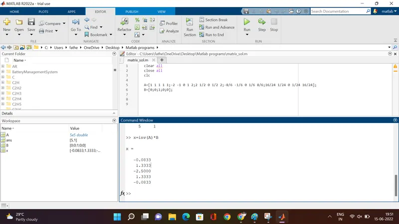
a=-0.0833
b=1.3333
c=-2.5000
d=1.3333
e=-0.0833

Here we see that a=e and b=d

Now dividing hypothesis equation(1) by `Deltax^2` we get

`(del^2u)/(delx^2) = (af(i-2)+b(i-1)+cf(i)+df(i+1)+ef(i+2))/(Deltax^2)`

Putting the values of a,b,c,d,e in above equation

`(del^2u)/(delx^2) = (-0.0833f(i-2)+1.3333f(i-1)-2.5000f(i)+1.3333f(i+1)-0.0833f(i+2))/(Deltax^2)`

From taylor table for second order derivative we get equation as

`(del^2u)/(delx^2)=(a+b+c+d+e)f(i)+(-2a-b+0+d+2e)f'(i)Deltax+(2a+b/2+0+d/2+2e)f''(i)Deltax^2+(-8a/6-b/6+0+d/6+8e/6)f'''(i)Deltax^3+(16a/24+b/24+0+d/24+16e/24)f''''(i)Deltax^4+(-32a/120-b/120+0+d/120+32e/120)f'''''(i)Deltax^5+(64a/720+b/720+0+d/720+64e/720)f''''''(i)Deltax^6`

To get 2nd order derivative the coefficient of f''(i) is 1 and f(i),f'(i),f'''(i),f''''(i) is 0 from equations 1,2,3,4,5 we get

`(del^2u)/(delx^2)=(2a+b/2+0+d/2+2e)f''(i)Deltax^2+(-32a/120-b/12+32e/120)f'''''(i)Deltax^5+(64a/720+b/720+0+d/720+64e/720)f''''''(i)Deltax^6`

In the above equation f'''''(i) term becomes 0 as a=e and b=d they get cancelled and dividing the remaining equation with `Deltax^2` we get

`(del^2u)/(delx^2)=(2a+b/2+0+d/2+2e)f''(i)++(64a/720+b/720+0+d/720+64e/720)f''''''(i)Deltax^4`

in the above equation `Deltax^4` denotes the truncation error and its order is 4. And we know that order of approximation is defined by truncation error term.So, for central difference method is 4th order accurate.

Putting the values of a,b,c,d,e in above equation the resultant equation is as follows

`(del^2u)/(delx^2)=(2(-0.0833)+1.3333/2+1.3333/2+2(-0.0833)f''(i)++((64/720)(-0.0833)+1.3333/720+(-0.0833)/720+(64/720)(-0.0833))f''''''(i)Deltax^4`

2.SKEWED RIGHT SIDE DIFFERENCE METHOD:

The numerical stencils for skewed right side difference method looks as follows

Here 4th order approximation is being computed at i taking 5 points surrounding right of i, let the points be (i+1),(i+2),(i+3),(i+4) and (i+5) and distance between them is `Deltax`.

The Stencil hypothesis equation is as follows

`(del^2u)/(delx^2) = af(i)+bf(i+1)+c(i+2)+df(i+3)+ef(i+4)+gf(i+5)` ... equation(1)

To find the values of a,b,c,d,e the taylor series expansion for equation(1) is as follows

For af(i)

`af(i)=af(i)`

For bf(i+1)

`bf(i+1)=bf(i)+b(f'(i)Deltax)/(1!)+b(f''(i)(Deltax)^2)/(2!)+b(f'''(i)(Deltax)^3)/(3!)+b(f''''(i)(Deltax)^4)/(4!)+b(f'''''(i)(Deltax)^5)/(5!)+b(f''''''(i)(Deltax)^6)/(6!)-....`

For cf(i+2)

`cf(i+2)=cf(i)+c(f'(i)2Deltax)/(1!)+c(f''(i)(2Deltax)^2)/(2!)+c(f'''(i)(2Deltax)^3)/(3!)+c(f''''(i)(2Deltax)^4)/(4!)+c(f'''''(i)(2Deltax)^5)/(5!)+c(f''''''(i)(2Deltax)^6)/(6!)-....`

For df(i+3)

`d(i+3)=df(i)+d(f'(i)3Deltax)/(1!)+d(f''(i)(3Deltax)^2)/(2!)+d(f'''(i)(3Deltax)^3)/(3!)+d(f''''(i)(3Deltax)^4)/(4!)+d(f'''''(i)(3Deltax)^5)/(5!)+d(f''''''(i)(3Deltax)^6)/(6!)-...`

For ef(i+4)

`e(i+4)=ef(i)+e(f'(i)4Deltax)/(1!)+e(f''(i)(4Deltax)^2)/(2!)+e(f'''(i)(4Deltax)^3)/(3!)+e(f''''(i)(4Deltax)^4)/(4!)+e(f'''''(i)(4Deltax)^5)/(5!)+e(f''''''(i)(4Deltax)^6)/(6!)-...`

For gf(i+5)

`g(i+5)=gf(i)+g(f'(i)5Deltax)/(1!)+g(f''(i)(5Deltax)^2)/(2!)+g(f'''(i)(5Deltax)^3)/(3!)+g(f''''(i)(5Deltax)^4)/(4!)+g(f'''''(i)(5Deltax)^5)/(5!)+g(f''''''(i)(5Deltax)^6)/(6!)-...`

Arranging the above expansion in Taylors table as follows

For the table we assume first six terms as, 1 for the required order i.e here for 2nd order and 0 for the 1st,2nd,4th,5th and 6th and for 7th we can't exactly define as 0 or 1.

From the above table we have 6equations forming as follows

`a+b+c+d+e+g=0`.....(1)

`b+2c+3d+4e+5g=0`.....(2)

`b/2+2c+(9d)/2+(16e)/2+(25g)/2=1`.....(3)

`b/6+(8c)/6+(27d)/6+(64e)/6+(125g)/6=0`......(4)

`b/24+(16c)/24+(81d)/24+(256e)/24+(625e)/24=0`.....(5)

`b/120+(32c)/120+(243d)/120+(1024e)/120+(3125g)/120=0`.....(6)

Writing it into matrix equation form of AX=B

`[[1,1,1,1,1,1],[0,1,2,3,4,5],[0,1/2,2,9/2,16/2,25/2],[0,1/6,8/6,27/6,64/6,125/6],[0,1/24,16/24,81/24,256/24,625/24],[0,1/120,32/120,243/120,1024/120,3125/120]]*[[a],[b],[c],[d],[e],[g]]=[[0],[0],[1],[0],[0],[0]]`

Solving above matrix in MATLAB we get

a=3.7500
b=-12.8333
c=17.8333
d=-13.0000
e=5.0833
g=-0.8333

Now dividing hypothesis equation(1) by `Deltax^2` we get

`(del^2u)/(delx^2)=(af(i)+bf(i+1)+c(i+2)+df(i+3)+ef(i+4)+gf(i+5))/(Deltax^2)`

Putting the values of a,b,c,d,e in above equation

`(del^2u)/(delx^2)=((3.7500)f(i)+(-12.8333)f(i+1)+(17.8333)(i+2)+(-13.0000)f(i+3)+(5.0833)f(i+4)+(-0.8333)f(i+5))/(Deltax^2)`

From taylor table for second order derivative we get equation as

`(del^2u)/(delx^2)=(a+b+c+d+e+g)f(i)+(b+2c+3d+4e+5g)f'(i)Deltax+(b/2+2c+(9d)/2+(16e)/2+(25g)/2)f''(i)Deltax^2+(b/6+(8c)/6+(27d)/6+(64e)/6+(125g)/6)f'''(i)Deltax^3+(b/24+(16c)/24+(81d)/24+(256e)/24+(625e)/24)f''''(i)Deltax^4+(b/120+(32c)/120+(243d)/120+(1024e)/120+(3125g)/120)f'''''(i)Deltax^5+(b/720+(64c)/720+(729d)/720+(4096e)/720+(15625g)/720)f''''''(i)Deltax^6`

To get 2nd order derivative the coefficient of f''(i) is 1 and f(i),f'(i),f'''(i),f''''(i),f'''''(i) is 0 from equations 1,2,3,4,5,6 we get

`(del^2u)/(delx^2)=(b/2+2c+(9d)/2+(16e)/2+(25g)/2)f''(i)Deltax^2+(b/720+(64c)/720+(729d)/720+(4096e)/720+(15625g)/720)f''''''(i)Deltax^6`

dividing the above equation with `Deltax^2` we get

`(del^2u)/(delx^2)=(b/2+2c+(9d)/2+(16e)/2+(25g)/2)f''(i)+(b/720+(64c)/720+(729d)/720+(4096e)/720+(15625g)/720)f''''''(i)Deltax^4`

in the above equation `Deltax^4` denotes the truncation error and its order is 4. And we know that order of approximation is defined by truncation error term.So, for central difference method is 4th order accurate.

Putting the values of a,b,c,d,e,g in above equation the resultant equation is as follows

`(del^2u)/(delx^2)=((-12.8333)/2+2(17.8333)+(9(-13.0000))/2+(16(5.0833))/2+(25(-0.8333))/2)f''(i)+((-12.8333)/720+(64(17.8333))/720+(729(-13.000))/720+(4096(5.0833))/720+(15625(-0.8333))/720)f''''''(i)Deltax^4`

2.SKEWED LEFT SIDE DIFFERENCE METHOD:

The numerical stencils for skewed left side difference method looks as follows

Here 4th order approximation is being computed at i taking 5 points surrounding left of i, let the points be (i-1),(i-2),(i-3),(i-4) and (i-5) and distance between them is `Deltax`.

The Stencil hypothesis equation is as follows

`(del^2u)/(delx^2) = af(i-5)+bf(i-4)+c(i-3)+df(i-2)+ef(i-1)+gf(i)` ... equation(1)

To find the values of a,b,c,d,e the taylor series expansion for equation(1) is as follows

For af(i-5)

`a(i-5)=af(i)-a(f'(i)5Deltax)/(1!)+a(f''(i)(5Deltax)^2)/(2!)-a(f'''(i)(5Deltax)^3)/(3!)+a(f''''(i)(5Deltax)^4)/(4!)-a(f'''''(i)(5Deltax)^5)/(5!)+a(f''''''(i)(5Deltax)^6)/(6!)-...`

For bf(i-4)

`b(i-4)=bf(i)-b(f'(i)4Deltax)/(1!)+b(f''(i)(4Deltax)^2)/(2!)-b(f'''(i)(4Deltax)^3)/(3!)+b(f''''(i)(4Deltax)^4)/(4!)-b(f'''''(i)(4Deltax)^5)/(5!)+b(f''''''(i)(4Deltax)^6)/(6!)-...`

For cf(i-3)

`c(i-3)=cf(i)-c(f'(i)3Deltax)/(1!)+c(f''(i)(3Deltax)^2)/(2!)-c(f'''(i)(3Deltax)^3)/(3!)+c(f''''(i)(3Deltax)^4)/(4!)-c(f'''''(i)(3Deltax)^5)/(5!)+c(f''''''(i)(3Deltax)^6)/(6!)-...`

For df(i-2)

`df(i-2)=df(i)-d(f'(i)2Deltax)/(1!)+d(f''(i)(2Deltax)^2)/(2!)-d(f'''(i)(2Deltax)^3)/(3!)+d(f''''(i)(2Deltax)^4)/(4!)-d(f'''''(i)(2Deltax)^5)/(5!)+d(f''''''(i)(2Deltax)^6)/(6!)-....`

For ef(i-1)

`ef(i-1)=ef(i)-e(f'(i)Deltax)/(1!)+e(f''(i)(Deltax)^2)/(2!)-e(f'''(i)(Deltax)^3)/(3!)+e(f''''(i)(Deltax)^4)/(4!)-e(f'''''(i)(Deltax)^5)/(5!)+e(f''''''(i)(Deltax)^6)/(6!)-....`

For gf(i)

`gf(i)=gf(i)`

Arranging the above expansion in Taylors table as follows

For the table we assume first six terms as, 1 for the required order i.e here for 2nd order and 0 for the 1st,2nd,4th,5th and 6th and for 7th we can't exactly define as 0 or 1.

From the above table we have 6equations forming as follows

`a+b+c+d+e+g=0`.....(1)

`-5a-4b-3c-2d-e=0`.....(2)

`(25a)/2+(16b)/2+(9c)/2+(2d)+(e)/2=1`.....(3)

`(-125a)/6-(64b)/6-(27c)/6-(8d)/6-(e)/6=0`......(4)

`(625a)/24+(256b)/24+(81c)/24+(16d)/24+(e)/24=0`.....(5)

`(-3125a)/120-(1024b)/120-(243c)/120-(32d)/120-(e)/120=0`.....(6)

Writing it into matrix equation form of AX=B

`[[1,1,1,1,1,1],[-5,-4,-3,-2,-1,0],[25/2,16/2,9/2,2,1/2,0],[-125/6,-64/6,-27/6,-8/6,-1/6,0],[625/24,256/24,81/24,16/24,1/24,0],[-3125/120,-1024/120,-243/120,-32/120,-1/120,0]]*[[a],[b],[c],[d],[e],[g]]=[[0],[0],[1],[0],[0],[0]]`

Solving above matrix in MATLAB we get

a=-0.8333
b=5.0833
c=-13.0000
d=17.8333
e=-12.8333
g=3.7500

Now dividing hypothesis equation(1) by `Deltax^2` we get

`(del^2u)/(delx^2)=(af(i-5)+bf(i-4)+c(i-3)+df(i-2)+ef(i-1)+gf(i))/(Deltax^2)`

Putting the values of a,b,c,d,e in above equation

`(del^2u)/(delx^2)=((-0.8333)f(i-5)+(5.0833)f(i-4)+(-13.0000)(i-3)+(17.8333)f(i-2)+(-12.8333)f(i-1)+(3.7500)f(i))/(Deltax^2)`

From taylor table for second order derivative we get equation as

`(del^2u)/(delx^2)=(a+b+c+d+e+g)f(i)+(-5a-4b-3c-2d-e)f'(i)Deltax+((25a)/2+(16b)/2+(9c)/2+(2d)+(e)/2)f''(i)Deltax^2+((-125a)/6-(64b)/6-(27c)/6-(8d)/6-(e)/6)f'''(i)Deltax^3+((625a)/24+(256b)/24+(81c)/24+(16d)/24+(e)/24)f''''(i)Deltax^4+(b/120+(-3125a)/120-(1024b)/120-(243c)/120-(32d)/120-(e)/120)f'''''(i-1)Deltax^5+((15625a)/720+(4096b)/720+(729c)/720+(64d)/720+(e)/720)f''''''(i)Deltax^6`

To get 2nd order derivative the coefficient of f''(i) is 1 and f(i),f'(i),f'''(i),f''''(i),f'''''(i) is 0 from equations 1,2,3,4,5,6 we get

`(del^2u)/(delx^2)=((25a)/2+(16b)/2+(9c)/2+(2d)+(e)/2)f''(i)Deltax^2+((15625a)/720+(4096b)/720+(729c)/720+(64d)/720+(e)/720)f''''''(i)Deltax^6`

dividing the above equation with `Deltax^2` we get

`(del^2u)/(delx^2)=((25a)/2+(16b)/2+(9c)/2+(2d)+(e)/2)f''(i)+((15625a)/720+(4096b)/720+(729c)/720+(64d)/720+(e)/720)f''''''(i)Deltax^4`

in the above equation `Deltax^4` denotes the truncation error and its order is 4. And we know that order of approximation is defined by truncation error term.So, for central difference method is 4th order accurate.

Putting the values of a,b,c,d,e,g in above equation the resultant equation is as follows

`(del^2u)/(delx^2)=((25(-0.8333))/2+(16(5.0833))/2+(9(-13.0000))/2+(2(17.8333))+(-12.8333)/2)f''(i)+((15625(-0.8333))/720+(4096(5.0833))/720+(729(-13.0000))/720+(64(17.8333))/720+(-12.8333)/720)f''''''(i)Deltax^4`

CODE FOR CENTRAL DIFFERENCE

function out = central_difference(x,dx)

%Analytical function given is f(x)=exp(x)*cos(x)

%Analytical derivative is f''(x) = -2*exp(x)*sin(x)

Analytical_derivative= -2*exp(x)*sin(x);

%values of coefficients of hypothesis equation

a=-0.0833;

b=1.3333;

c=-2.5000;

d=1.3333;

e=-0.0833;

%Numerical derivative

%central

%differencing=((a*f(x-2*dx))+(b*f(x-dx))+(c*f(x))+(d*f(x+dx))+(e*f(x+2*dx)))/dx^2

central_differencing = ((a*exp(x-2*dx)*cos(x-2*dx))+(b*exp(x-dx)*cos(x-dx))+(c*exp(x)*cos(x))+(d*exp(x+dx)*cos(x+dx))+(e*exp(x+2*dx)*cos(x+2*dx)))/(dx^2);

out = abs(central_differencing-Analytical_derivative);

end

STEPS:

1.The analytical derivative is defined

2.The coefficients for the hypothesis i.e values of a,b,c,d,e are given

3.The central differnce equation is defined

4.The error is calculated from Analytical derivative using absolute command

CODE FOR RIGHT SKEWED DIFFERENCE

function out = right_skewed_difference(x,dx)

%Analytical function given is f(x)=exp(x)*cos(x)

%Analytical derivative is f''(x) = -2*exp(x)*sin(x)

Analytical_derivative= -2*exp(x)*sin(x);

%values of coefficients of hypothesis equation

a=3.7500;

b=-12.8333;

c=17.8333;

d=-13.0000;

e=5.0833;

g=-0.8333;

%Numerical derivative

%skewed right differencing=((a*f(x))+(b*f(x+1))+(c*f(x+2))+(d*f(x+3))+(e*f(x+4))+(g*f(x+5)))/dx^2

Right_skewed_difference = ((a*exp(x)*cos(x))+(b*exp(x+dx)*cos(x+dx))+(c*exp(x+2*dx)*cos(x+2*dx))+(d*exp(x+3*dx)*cos(x+3*dx))+(e*exp(x+4*dx)*cos(x+4*dx))+(g*exp(x+5*dx)*cos(x+5*dx)))/(dx^2);

out = abs(Right_skewed_difference-Analytical_derivative);

end

STEPS:

1.The analytical derivative is defined

2.The coefficients for the hypothesis i.e values of a,b,c,d,e,g are given

3.The right skewed differnce equation is defined

4.The error is calculated from Analytical derivative using absolute command

CODE FOR LEFT SKEWED DIFFERENCE

function out = left_skewed_difference(x,dx)

%Analytical function given is f(x)=exp(x)*cos(x)

%Analytical derivative is f''(x) = -2*exp(x)*sin(x)

Analytical_derivative= -2*exp(x)*sin(x);

%values of coefficients of hypothesis equation

a=-0.8333;

b=5.0833;

c=-13.0000;

d=17.8333;

e=-12.8333;

g=3.7500;

%Numerical derivative

%skewed right differencing=((a*f(x-5))+(b*f(x-4))+(c*f(x-3))+(d*f(x-2))+(e*f(x-1))+(g*f(x)))/dx^2

Left_skewed_difference = ((a*exp(x-5*dx)*cos(x-5*dx))+(b*exp(x-4*dx)*cos(x-4*dx))+(c*exp(x-3*dx)*cos(x-3*dx))+(d*exp(x-2*dx)*cos(x-2*dx))+(e*exp(x-dx)*cos(x-dx))+(g*exp(x)*cos(x)))/(dx^2);

out = abs(Left_skewed_difference-Analytical_derivative);

end

STEPS:

1.The analytical derivative is defined

2.The coefficients for the hypothesis i.e values of a,b,c,d,e,g are given

3.The left skewed differnce equation is defined

4.The error is calculated from Analytical derivative using absolute command

MAIN CODE FOR TAYLOR TABLE

clear all

close all

clc

x = pi/3;

dx = linspace(pi/40,pi/4000,20); %given range for meshing

for i = 1:length(dx) %to begin the process for iteration declaring 'i'

%calling central_difference function

central_difference_error(i) = central_difference(x,dx(i));

%calling right_skewed_difference function

right_skewed_error(i) = right_skewed_difference(x,dx(i));

%calling left_skewed_difference

left_skewed_error(i) = left_skewed_difference(x,dx(i));

end

%Plotting the graph

figure(1)

loglog(dx,central_difference_error,'LineWidth',3,'Color','b');

hold on

loglog(dx,right_skewed_error,'LineWidth',3,'Color','r');

hold on

loglog(dx,left_skewed_error,'LineWidth',3,'Color','g');

xlabel('dx');

ylabel('Error');

legend('Central difference error','Right skewed error','Left skewed error');

STEPS:

1.The value for x and meshing range for dx is defined

2.The errors for central difference, right skewed difference and left skewed difference is calculated using for loop with using iterative steps

3.Plots are plotted w.r.t dx and the difference methods using loglog command

RESULTS:

From the above plot we can conclude that central difference method has minimum errors compared to other two difference methods.So, the central difference method is the most reliable method to use.

WHY SKEWED SCHEME IS USEFUL? WHAT CAN SKEWED SCHEME CAN DO THAT CD CANNOT:

The central method is more accurate and with minimum number of errors compared to other difference methods of skewed scheme but central difference method need the values before and after it to compute. While if we need to compute at right end of domain and we don't have any valued after the required derivative then we cannot compute by central differencing we need to go by skewed methods only to get the result.

CONCLUSION:

Thus the taylors table for central,right-skewed and left-skewed has been computed for 4th order with second derivative and the comparision for the same has been done using plotting the graph.