Week 2 Railwheel and Track
AIM: To perform a static structural analysis on the Railwheel and Track setup.
CASE_1 :
Perform a static structural analysis on the Railwheel and Track setup with the load of 100000 N, compare the results by multiplying the bearing load by 5 times . Compare the Total Deformation, Equivalent stress, and the life under both the loads.
CASE_2 :
Implement a User-defined result and calculate the Total Deformation from this result and check if it is the same as that obtained by the inbuilt result by ANSYS for a load of 100000 N. (Using an EXPRESSION find the User-defined result)
Theory:
Bearing load on wheel:
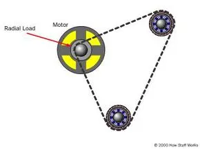
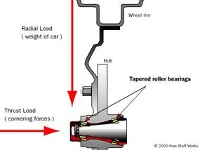
Bearings typically have to deal with two kinds of loading, radial and thrust. Depending on where the bearing is being used, it may see all radial loading, all thrust loading or a combination of both.
The bearings in the electric motor and the pulley pictured below face only a radial load. In this case, most of the load comes from the tension in the belt connecting the two pulleys.
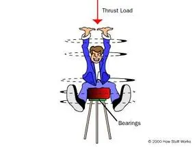
The bearing above is like the one in a barstool. It is loaded purely in thrust, and the entire load comes from the weight of the person sitting on the stool.
The bearing above is like the one in the hub of your car wheel. This bearing has to support both a radial load and a thrust load. The radial load comes from the weight of the car, the thrust load comes from the cornering forces when you go around a turn.
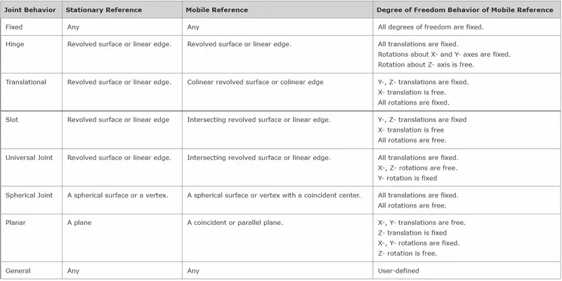
Types of joints:
Types of contacts:
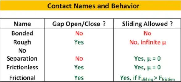
Contact behaviour:
Symmetric Behavior:
The Contact surfaces are constrained from penetrating the Target surfaces and the Target surfaces are constrained from penetrating the Contact surfaces.
Asymmetric Behavior:
Only the Contact surfaces are constrained from penetrating the Target surfaces.
Trim contact:
'Trim contact' and 'Pinball radius' are used to define the range for contact region.
Basically with trim contact active it removes contact and target elements that are outside of the user specified tolerance prior to solving.
A contact element is considered to be in near-field contact when its integration points (Gauss points or nodal points) are within a code-calculated (or user-defined) distance to the corresponding target surface. This distance is referred to as the pinball region. The pinball region is a circle (in 2-D) or a sphere (in 3-D) centered about the Gauss point.
So Pinball radius is used in solution and effects the contact and element status.
Interface treatment:
Add offset with 0 as the offset is the default for frictional or frictionless contact and is the correct one to use to have the pretension squeeze two flanges together.
Add Offset allows the user to specify any desired positive or negative distance to offset the contact surfaces. A positive value will tend to close a gap while a negative value will tend to open a gap.
Add Offset, Ramped Effects ramps the interference linearly over all substeps in the load step. This is a useful technique to enhance convergence for challenging interference problems.
Add Offset, No Ramping applies the interference all at once in first substep of the load step.
Procedure:
The CAD model of rail wheel and track setup:
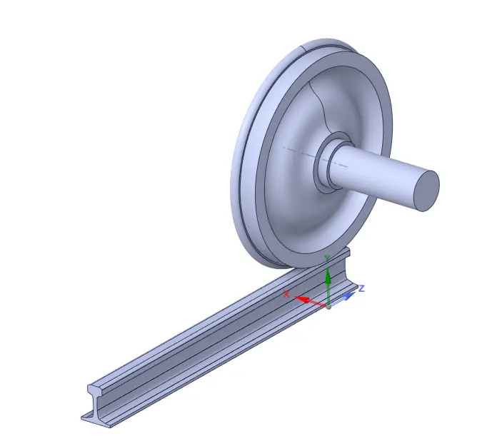
There are three main parts considered
1. Wheel
2. Rail
3. Shaft
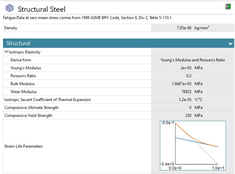
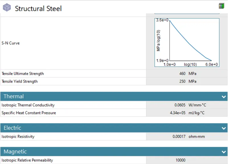
The material used is Structural Steel
The properties used are:
Contacts:
The contact is defined between the wheel and the track.
The type of contact is frictional with co-efficient of friction as 0.3
The interface treatment of Add offset, No ramping is used. This applies the interference all at once in first substep of the load step.
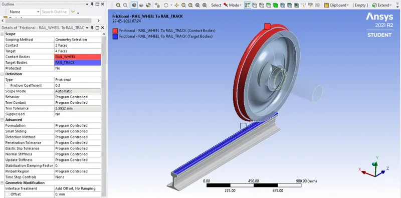
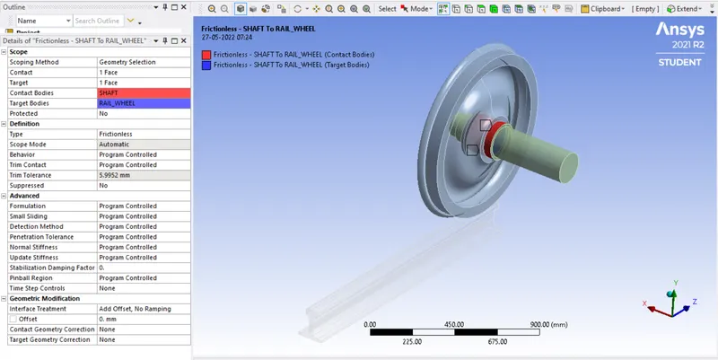
The frictionless contact is defined between the shaft and the wheel
Joints:
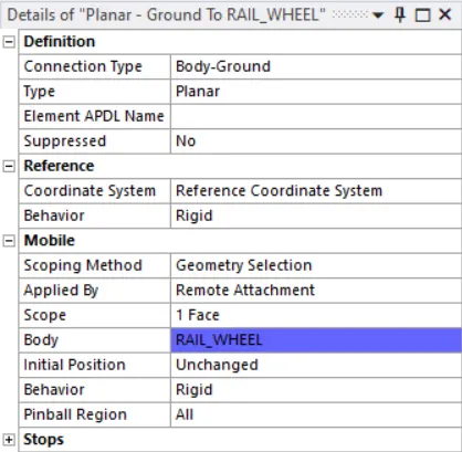
The planar joint is used to contain the wheel in the same plane w.r.t ground.
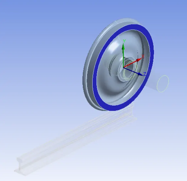
The rail is to be fixed at its position w.r.t ground.
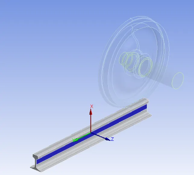
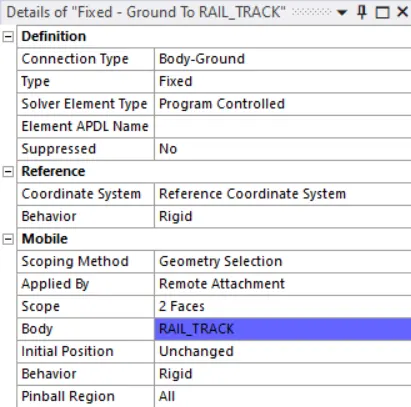
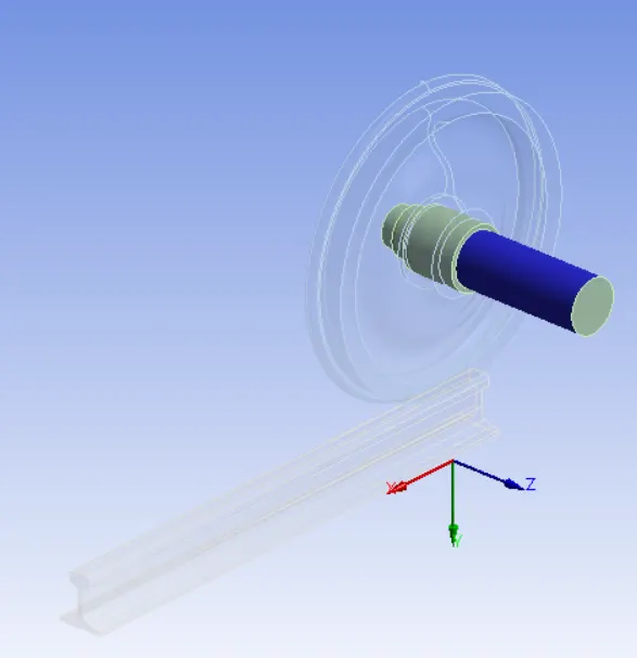
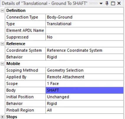
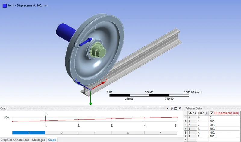
The translational joint is used for the shaft to obtain the motion of the wheel on the rail.
Mesh:
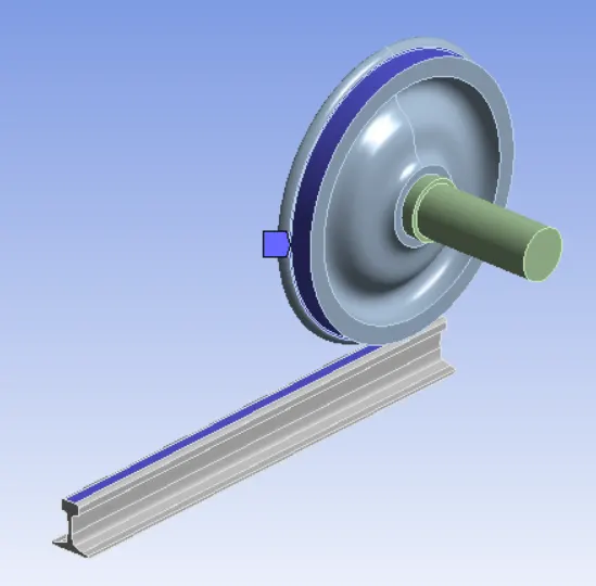
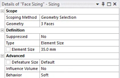
The mesh sizing is used to obtain the finer mesh of 35mm near the contact zone.
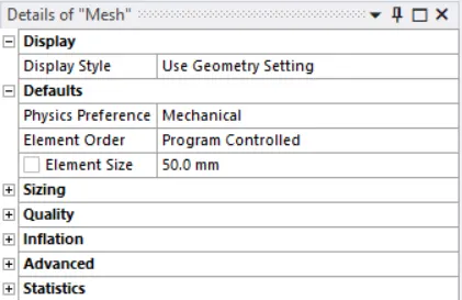
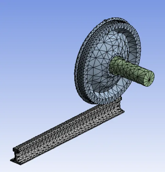
The mesh size of 50mm is used.
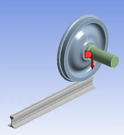
Bearing load:As there is no radial force that is generated we have only considered the thrust force on the wheel by the shaft and the load.
The load of 100000 N is applied.
The displacement is assigned to the translational joint. The tabular data of how displacement is varying over time is mentioned below
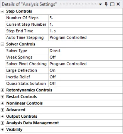
Analysis settings:
Total number of steps used in the simulation is 5 steps.
For the first step, Auto time stepping is program controlled. The direct solver is enabled. Turn the large deflection (For the non-linear problems, by turning on the large deflection changes in stiffness due to changes in the shape of the parts you are simulating are included)
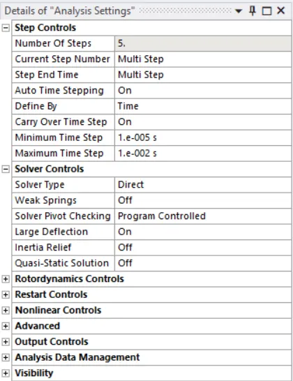
For the next four steps, Auto time stepping is enabled, Defined by the time (Time step criterion is mentioned)
Carry over time step is enabled(This enables the continuity in the time step w.r.t previous step)
The large deflection is turned on.
Request the necessary outputs and solve the problem.
Make use of 4 cores if available from the Solve process settings.
Results:
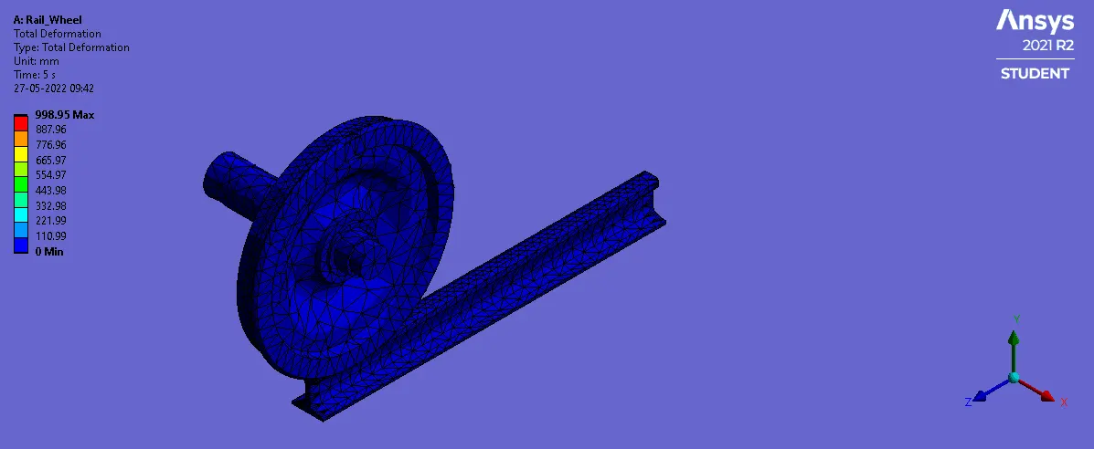
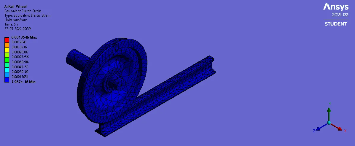
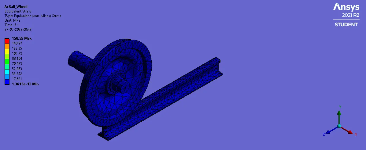
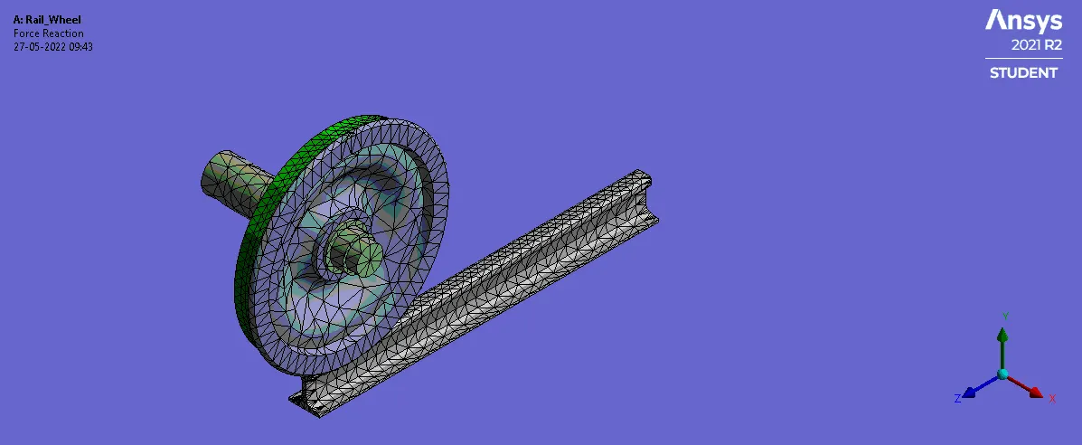
Results with the load of 100000 N
Total deformation:
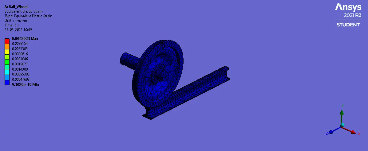
Equivalent Strain:
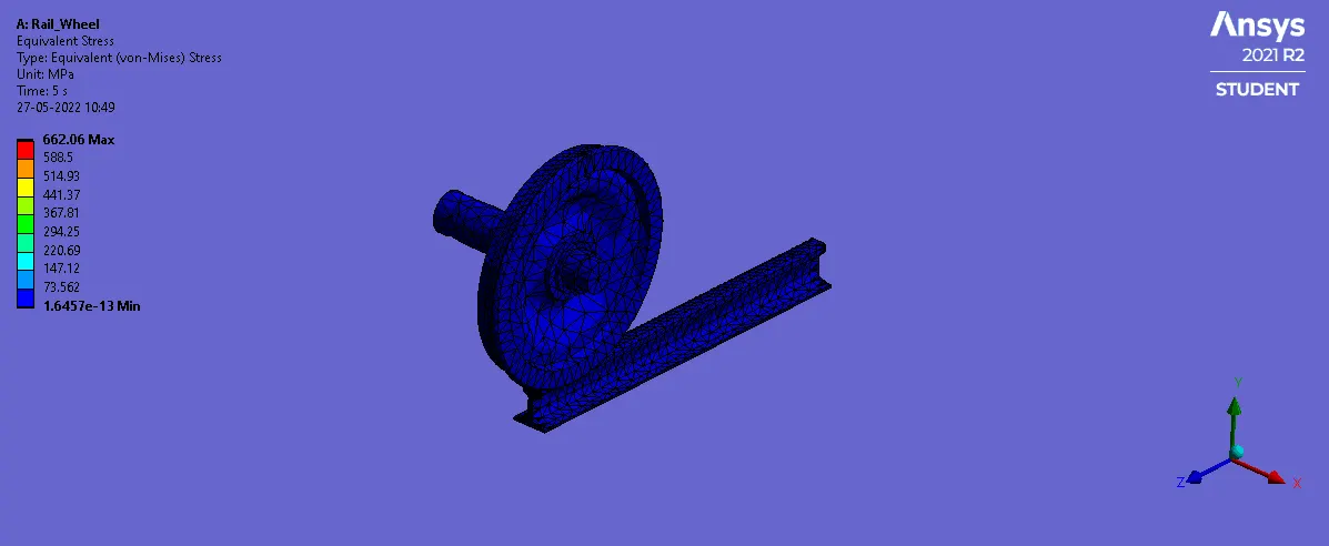
Equivalent Stress:
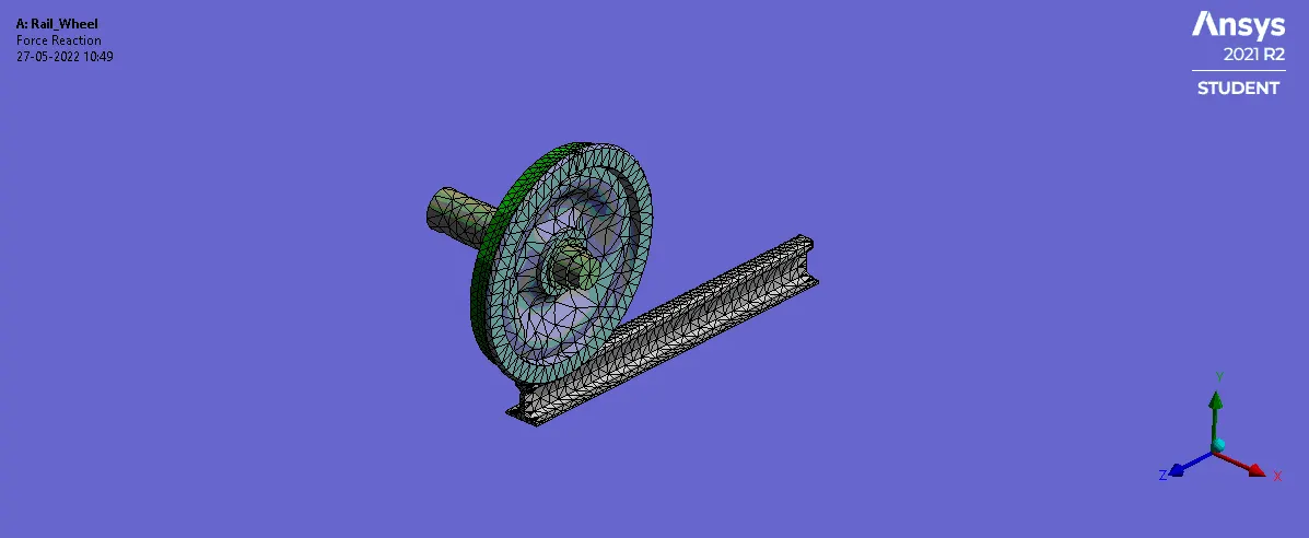
Force reaction:
Results with the load of 500000 N:
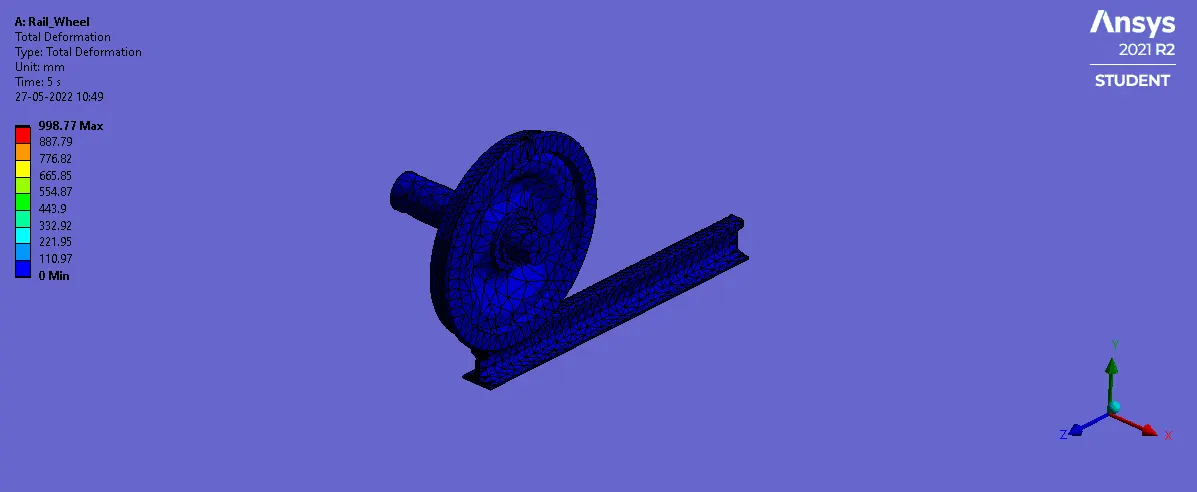
Total deformation:
Equivalent Strain:
Equivalent Stress:
Force reaction:
Comparision of the results:

Case_2:
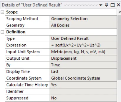
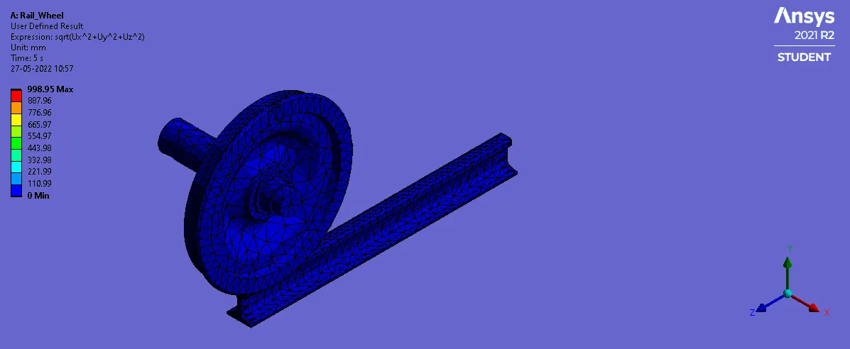
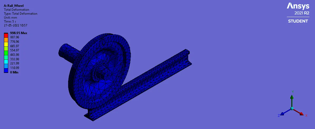
We can see that the total deformation calculated using the user defined expression is equal to the total deformation obtained from in-built by ANSYS for the load of 100000 N.
Conclusion:
- We can see the stress generated is 159 Mpa, deformation is 999 mm, and the life(fatigue life gives you a comprehensive diagnostic fatigue process to predict your product's operational lifetime.) is 6.02E+5 cycles for a bearing load of 1E+5 N.
- With increase in bearing load by 5 times, The deformation remained constant, the stress is increased to 662 Mpa which is almost 4 times, and the life of the components goes down to 3170 cycles.
- For the case-2, We can see that the total deformation calculated using the user defined expression is equal to the total deformation obtained from in-built by ANSYS for the load of 100000 N.