Week 2 Railwheel and Track
Week 2 Challenge: Rail Wheel and Track Challenge
Course: Structural Analysis Using Ansys Workbench
Submitted by: Amanpreet Singh Whan
Supervisor: Vineet G
March 02, 2022
List of Figures
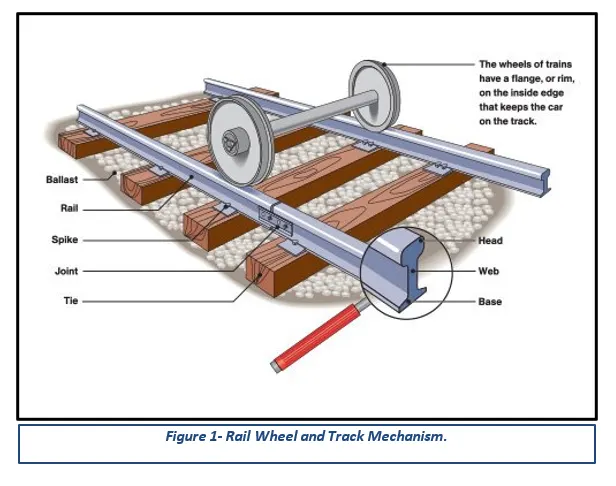
Figure 1- Rail Wheel and Track Mechanism.
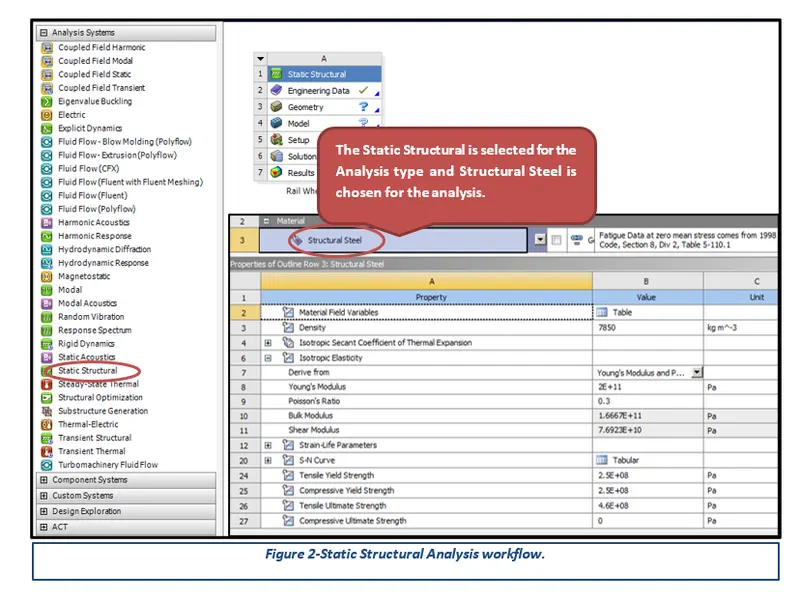
Figure 2-Static Structural Analysis workflow.
Figure 3-Imported given Rail Wheel Track CAD Model.
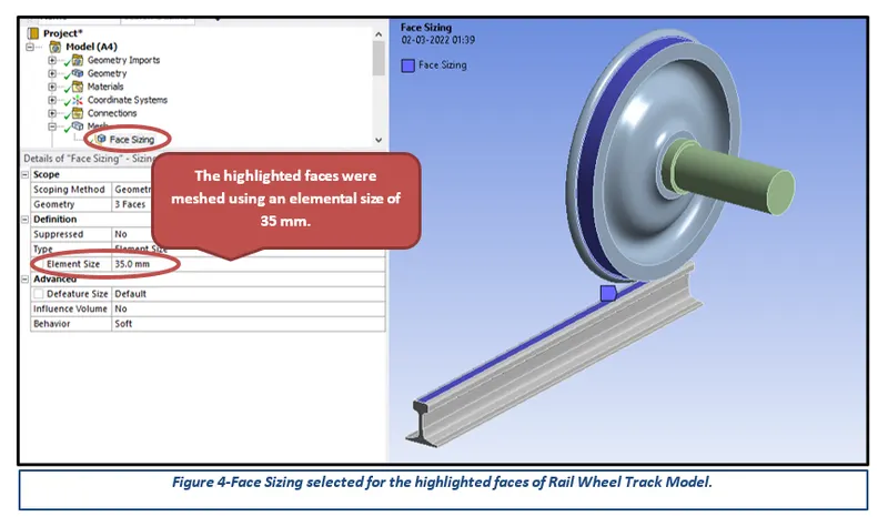
Figure 4-Face Sizing selected for the highlighted faces of Rail Wheel Track Model.
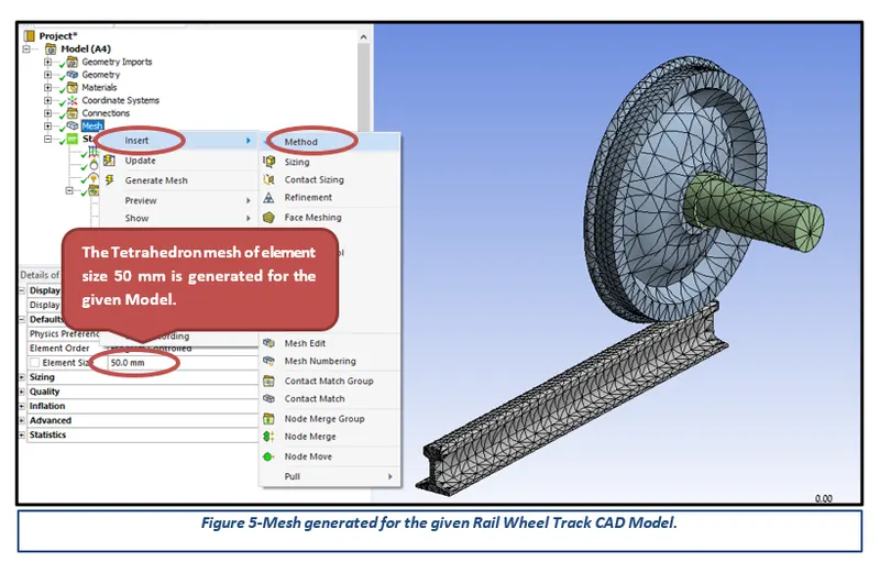
Figure 5-Mesh generated for the given Rail Wheel Track CAD Model.
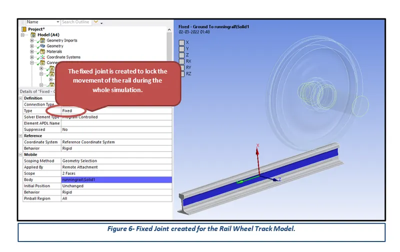
Figure 6- Fixed Joint created for the Rail Wheel Track Model.
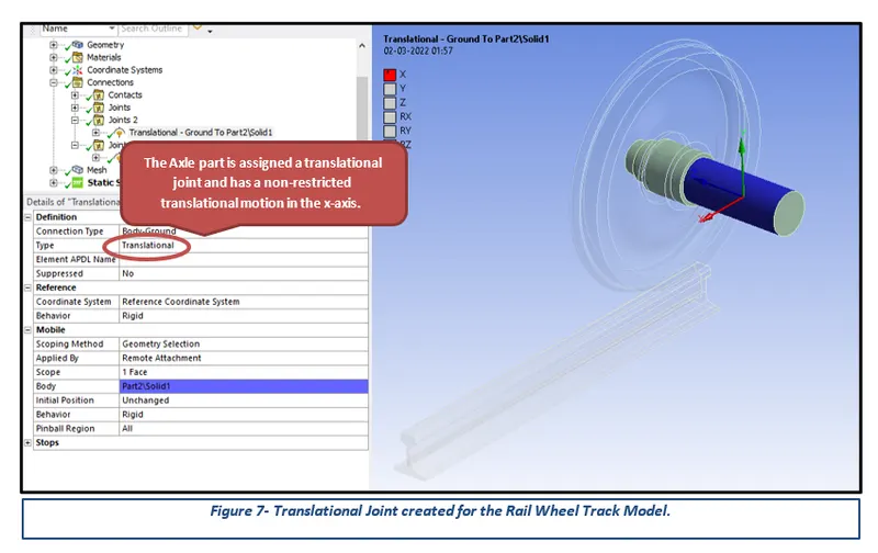
Figure 7- Translational Joint created for the Rail Wheel Track Model.
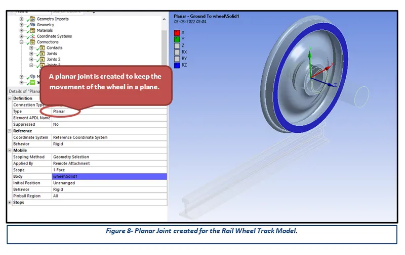
Figure 8- Planar Joint created for the Rail Wheel Track Model.
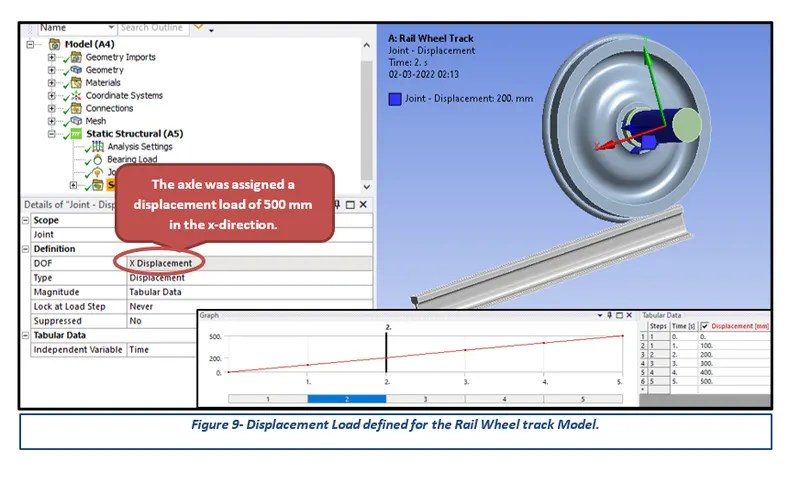
Figure 9- Displacement Load defined for the Rail Wheel track Model.
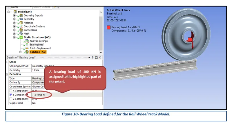
Figure 10- Bearing Load defined for the Rail Wheel track Model.
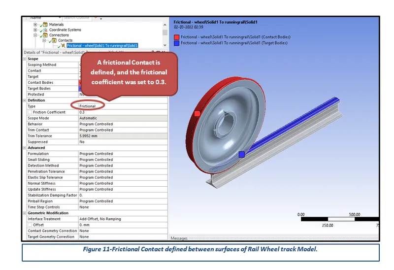
Figure 11-Frictional Contact defined between surfaces of Rail Wheel track Model.
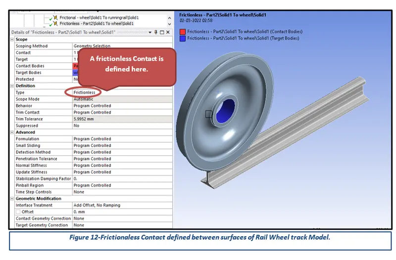
Figure 12-Frictionaless Contact defined between surfaces of Rail Wheel track Model.
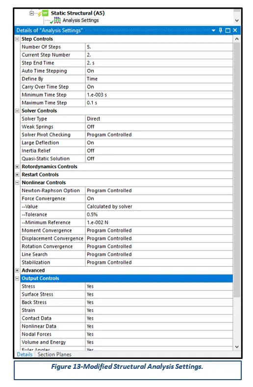
Figure 13-Modified Structural Analysis Settings.
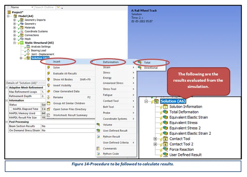
Figure 14-Procedure to be followed to calculate results.
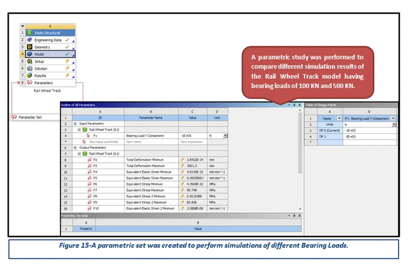
Figure 15-A parametric set was created to perform simulations of different Bearing Loads.
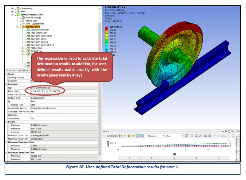
Figure 16- User-defined Total Deformation results for case 1.
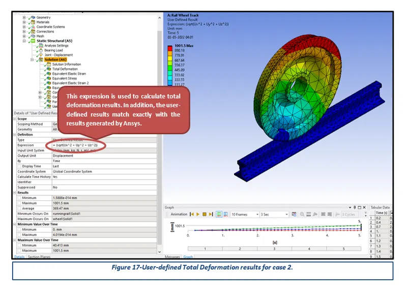
Figure 17-User-defined Total Deformation results for case 2.
Table of Contents
3.1 Importing and Meshing of CAD Model
1 Introduction
ANSYS is a general-purpose, finite-element modeling package for numerically solving a wide variety of mechanical problems. These problems include static/dynamic, structural analysis, heat transfer, and fluid problems, as well as acoustic and electromagnetic problems. There are two methods to use ANSYS. One method is to use the graphical user interface (GUI). This method follows the conventions of popular Windows and X-Windows-based programs. Another method is to use command files. The command-file approach has a steeper learning curve for many, but it has the advantage that the entire analysis can be described in a small text file, typically in less than 50 lines of commands. This approach enables easy model modifications and minimal file-space requirements. The ANSYS environment contains two windows: the main window and an output window. A large number of files are created when ANSYS simulation is run.
Theory
There are roughly 25–50 million railway wheels in operation in the world today. Allowing an annual failure rate of one in 1000 would mean 25 000–50 000 failed wheels every year. It is quite clear that if ‘failure’ here refers to a complete fracture of the wheel causing the train to be inoperative, railways would not be an efficient means of transportation.
Most ‘failures’ due to wheel fatigue are less dramatic. In most cases, cracks are mitigated before they have become sufficiently large to cause catastrophic failures. Still, wheel fatigue may have major operational and economic consequences. The fact that wheel fatigue failures tend to come in ‘epidemics’ causing major operational disturbances further adds to this.
As we increase axle loads and train speeds together with the overall utilization of train fleets, wheel fatigue issues are bound to increase if countermeasures are not taken. Due to the massive number of operational wheels and the decreasing margins for operational errors, there is a vast potential in cost savings from improved wheel fatigue management. accidents caused by wheel fractures are rare. Though fatal accidents are even rare they are often highly publicized, which may cause customers to abandon train transportation. This has a highly negative consequence since a decrease in train transportation, whether due to questionable safety, decreased operational reliability, or reduced economic competitiveness draws passengers and freight to cars, trucks, and airplanes. All of these are inferior means of transportation from a socioeconomic, environmental, and safety point of view.
So, from an operational point of view, an understanding and implementation of knowledge on wheel fatigue are of significant importance. However, the subject is also interesting from a scientific point of view. Historically, railways and fatigue research have been closely linked. With the introduction of railways, dynamic loads of sufficient magnitude and duration to cause fatigue failures were introduced, and the first systematic study of metal fatigue was carried out on railway axles in the 1850s. Since then, a lot of knowledge has been gained, but fatigue in general, and fatigue of railway wheels is a problem that is still far from fully solved.
The challenge presents an FEA study of the Rail Wheel Track conducted using ANSYS to simulate approximate real-life fatigue analysis. A bearing load of 100 KN is applied to the wheel structure against rail (beam) structure to analyze total deformation and stress-strain results.
2 Aims
- Perform a static structural analysis on the given Rail wheel and Track CAD model.
- Apply appropriate Boundary Conditions and Joint Loads.
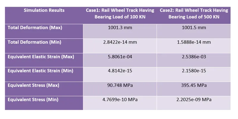
- Determine Total Deformation and Maximum Stress results for the performed simulations and compare the results for the same.
3 Methodology and Results
The section describes the different stages that were performed using an engineering tool Ansys Workbench 2022 for the completion of the Week 2 Challenge. These stages can be further broadly sub-categorized into three key steps, importing the CAD model to apply the boundary conditions and finally performing the simulation to obtain the desired results.
3.1 Importing and Meshing of CAD Model
After opening the Ansys Workbench, the first step is to select the Analysis type and then define appropriate material from the Engineering Data options for the given CAD model. Considering the challenge requirements, Static Structural was selected for the System Analysis type while Structural Steel was selected as a material for the challenge purposes. The following figures highlight the analysis system and material card parameters in detail.
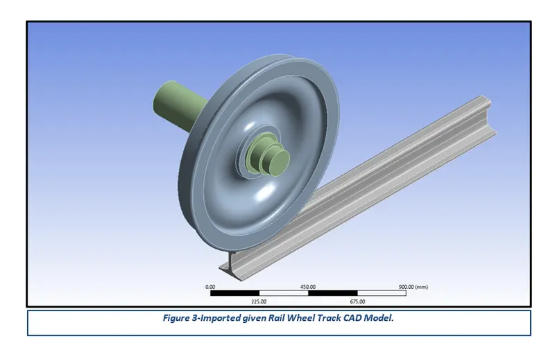
After updating the CAD model in the Ansys Workbench, the next step is to generate a good quality mesh. Meshing is a phase where the CAD geometry is discretized to represent the computational domain in which the solver will discover a solution. A refined mesh helps to achieve better results. The mesh was generated in two steps: a face sizing method with an element size of 35 mm was used to refine the faces in contact; for other areas, the mesh was generated using an element size of 50 mm.
3.2 Joints
A joint is a type of connection or junction at which usually two bodies are joined together in a way that restricts some degrees of freedom (DOFS) while leaving others free. For a joint, one reference is considered the stationary reference, while the other is considered the mobile or moving reference. The mobile and stationary references of the joint must be on two different bodies. Joints can also be defined as “grounded”. In this case, the joint connects the mobile reference to a fixed location in space. The stationary references are fixed in space, that is they have all DOFs fixed. Properties of a joint are defined as a joint behavior and can be applied to more than one joint. Joint behavior is characterized by the rotational and translational degrees of freedom of the mobile reference of the joint, as fixed or free concerning the stationary one.
The following figures represent the three joints created: Fixed joint, Translational joint, and Planar joint as per the challenge requirements.
3.3 Contact
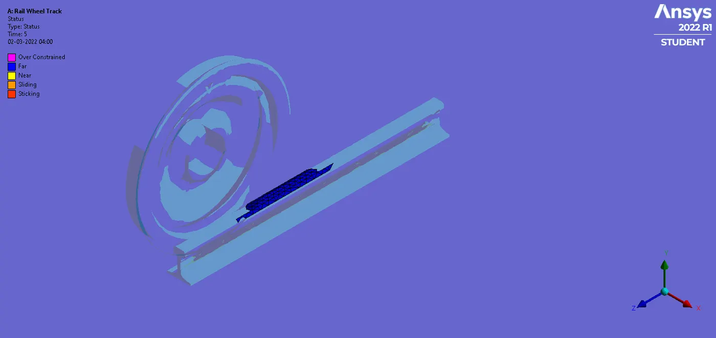
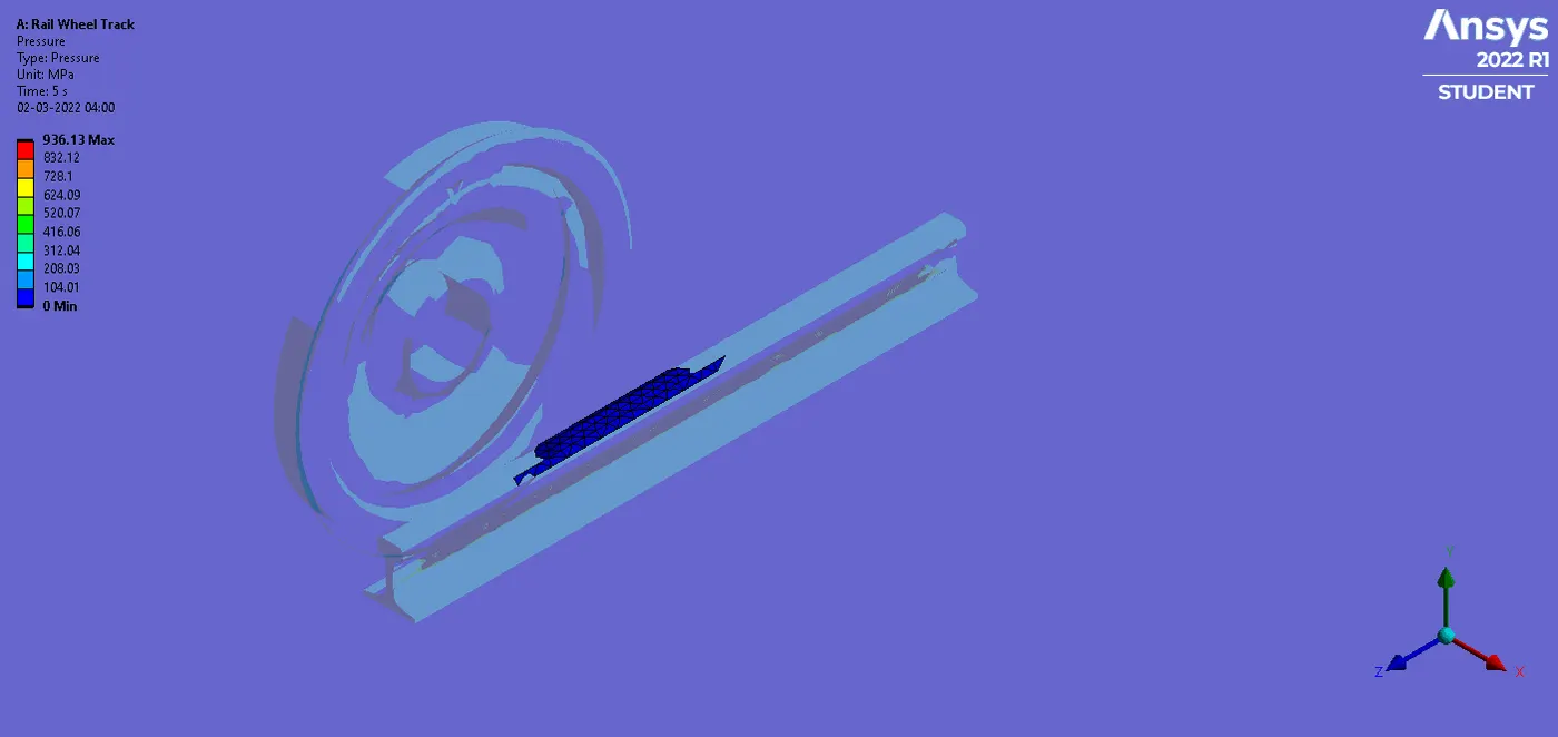
In structural analysis software, the contact is generated by pair. Three different contact behaviors are available. They are named node to node (point to point), node to a surface (point to the surface), and surface to surface. As default in Ansys software, point to surface and surface to surface contact types are used. For the point to surface contact, the “point” is contact, and the “surface” is the target. Several contact types are used. These names might be called with different names according to software. In Ansys software, contact names are titled frictional, frictionless, rough, bonded, and have no separation. The Frictional Contact and Frictionless contact were defined for the challenge purposes and are represented in the following figures.
3.4 Analysis Settings
The given spur gear model was assumed to be simulated for a translation of 500 mm to determine appropriate total deformation and other stress-strain results. Therefore, the problem was divided into 5 steps and the Large Deflection option was turned on to prevent Penetration and Intersection errors. The following figure represents the modifications performed in the analysis settings.
Simulation Results
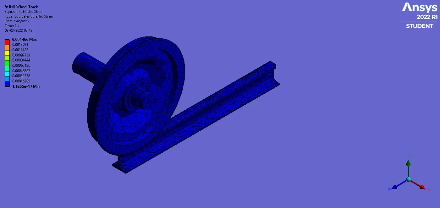
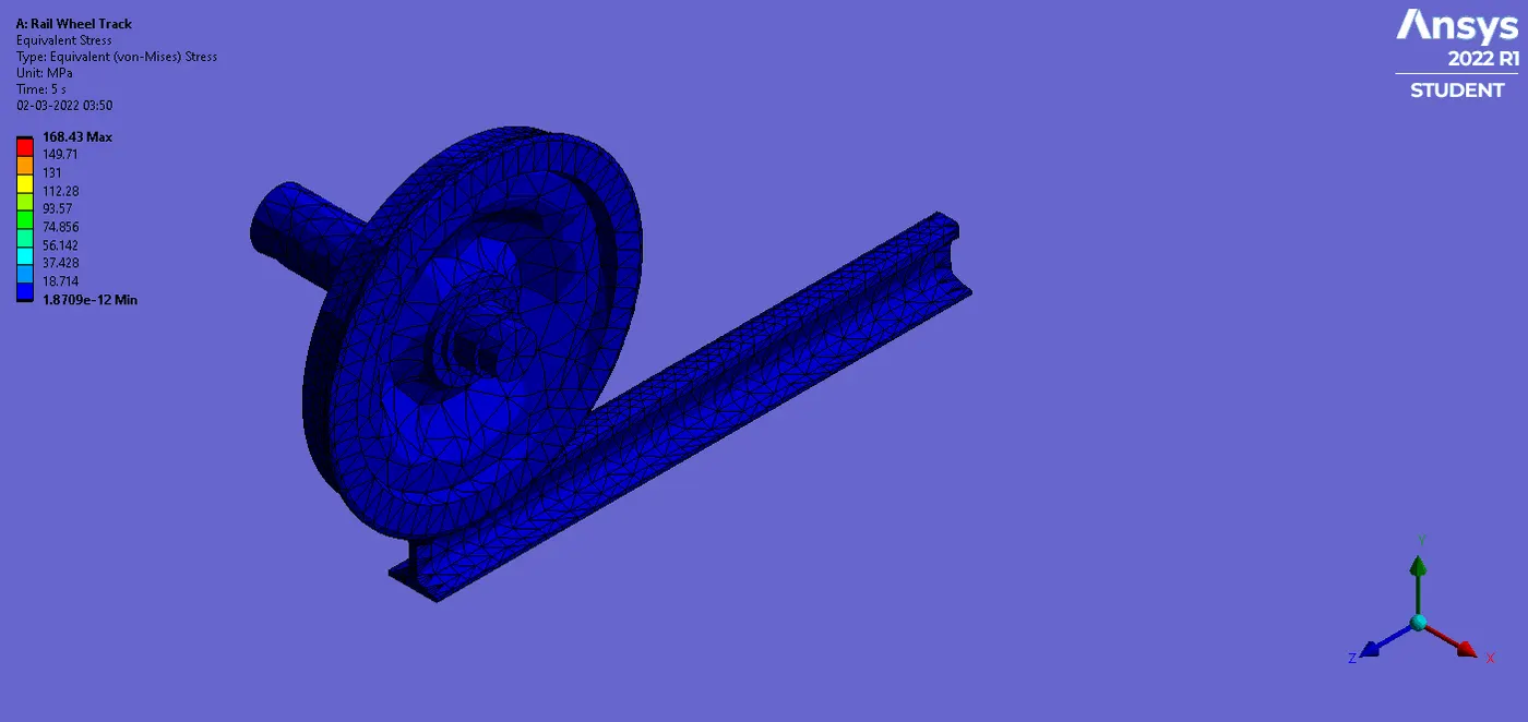
To visualize the simulation or results, the desired output cards have to be created. Total Deformation, Equivalent Elastic Strain, and Equivalent Stress (Von Mises Stress) cards were created using the procedure illustrated in the following picture. It must be noted that the results have to be generated by running the solve command.
A parametric study was created to find and compare the simulation results of the Rail Wheel Track model with different bearing loads of 100 KN and 500 KN. The created parametric set is highlighted in the following figure.
Case1: Simulation Results of Rail Wheel Track Model having Bearing Load of 100 KN
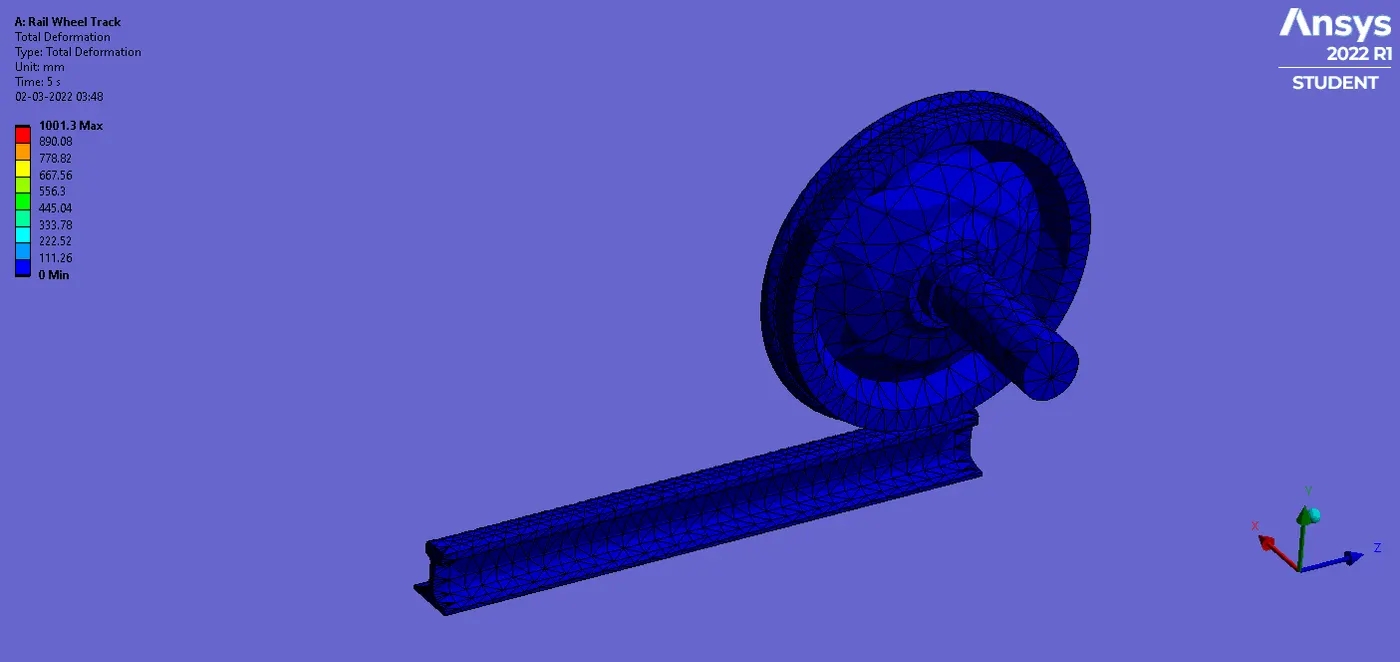
Total Deformation Results:
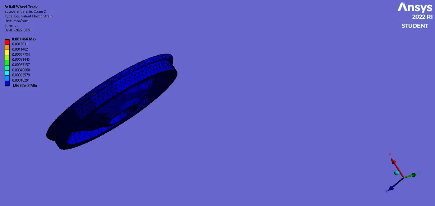
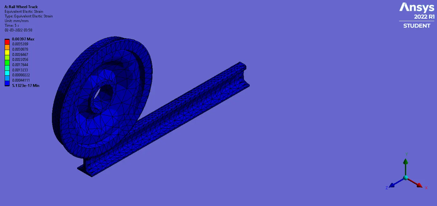
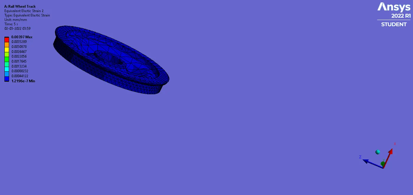
Stress-Strain Results:
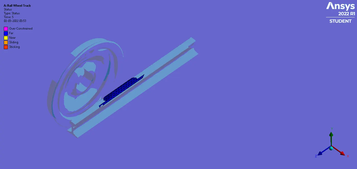
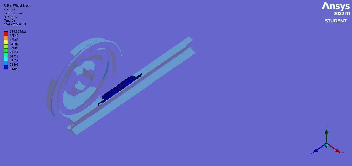
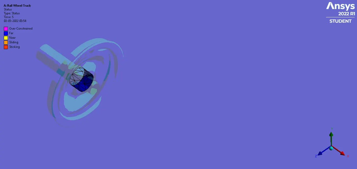
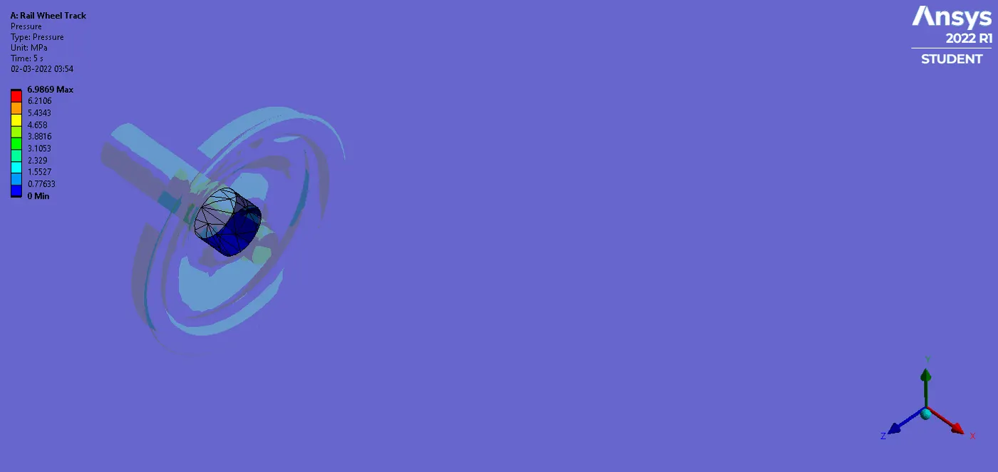
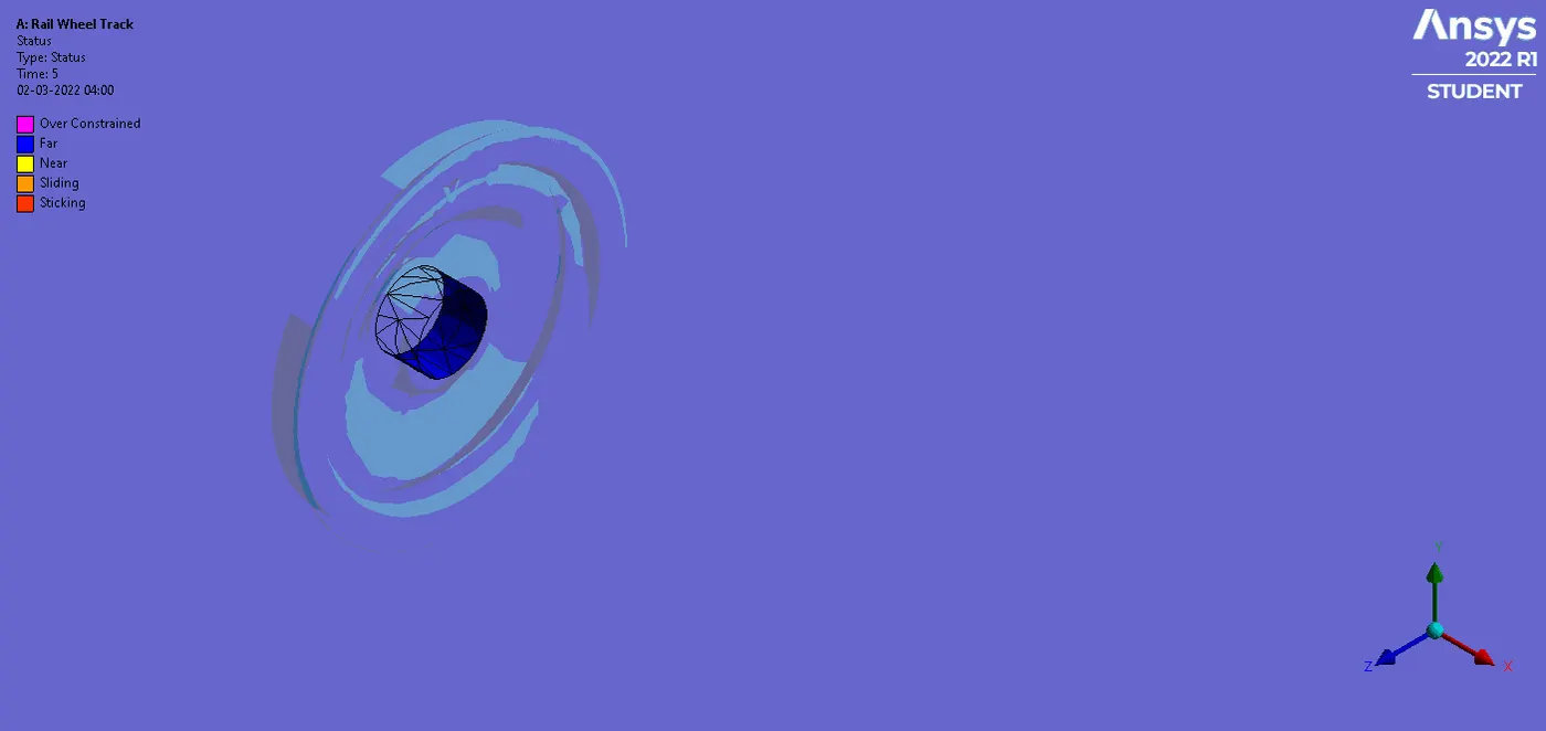
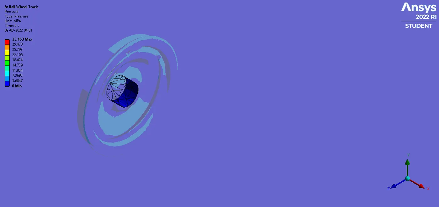
Contact Tool Results:
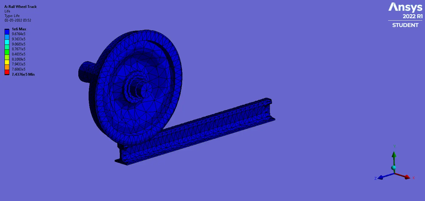
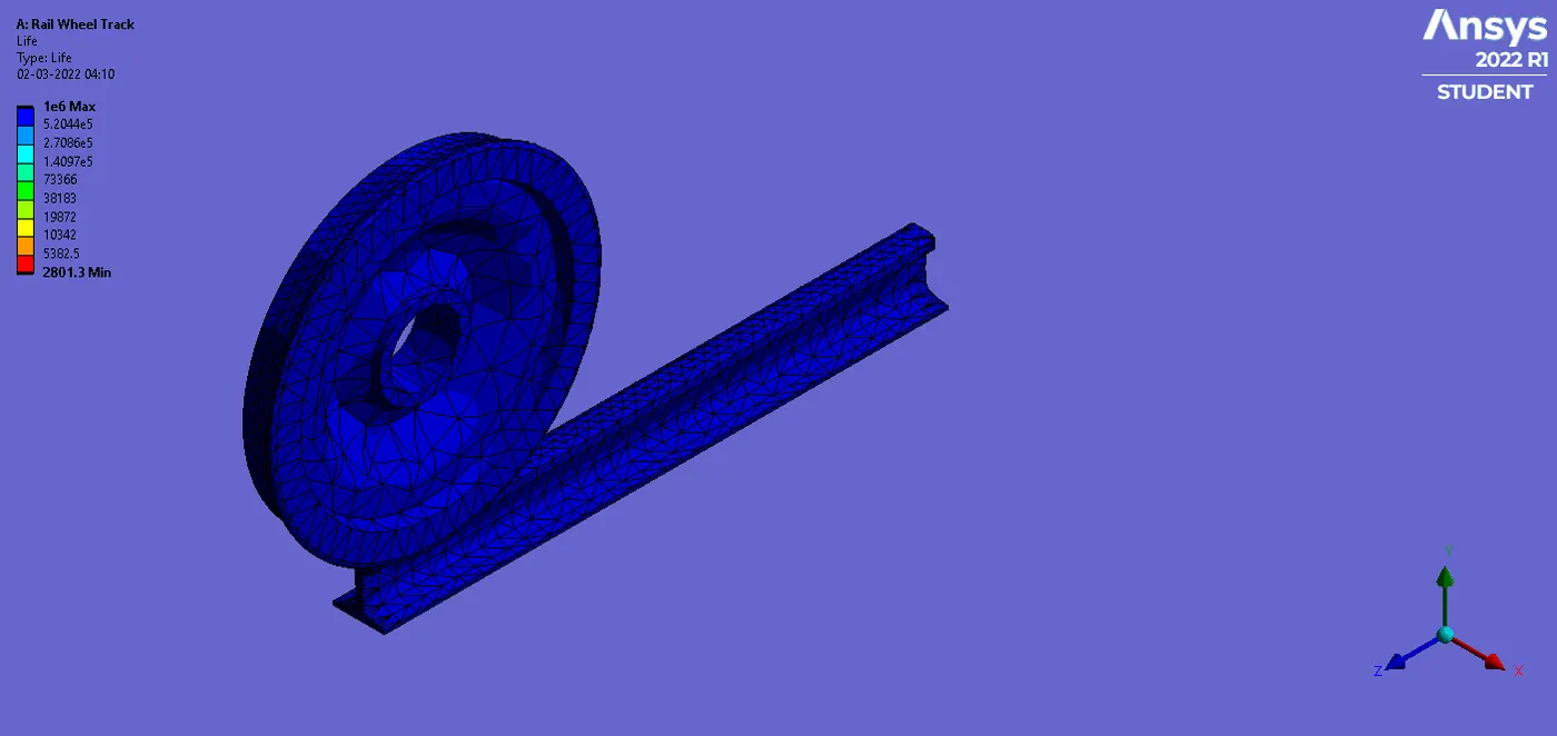
Fatigue Tool Results:
User-defined Total Deformation Results:
Case2: Simulation Results of Rail Wheel Track Model having Bearing Load of 500 KN
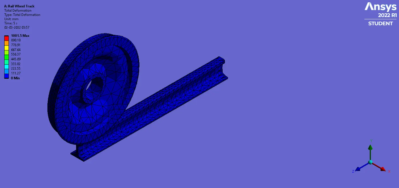
Total Deformation Results:
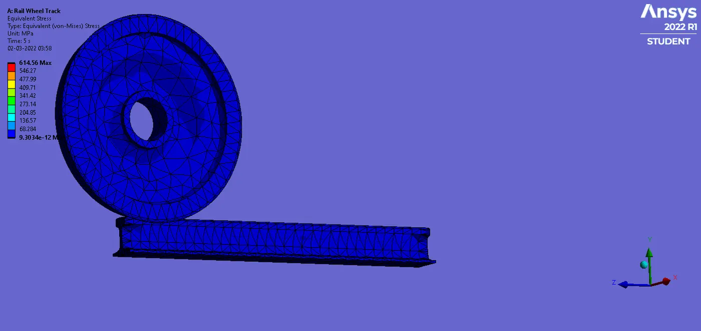
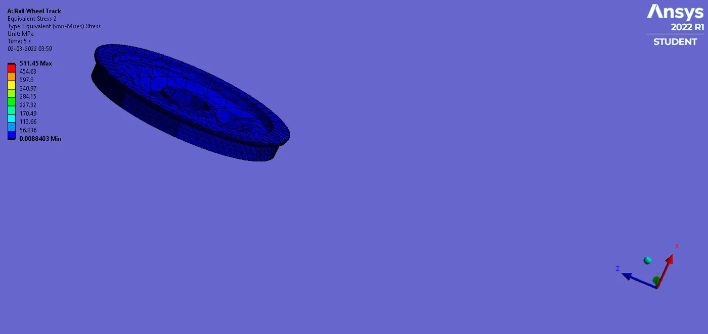
Stress-Strain Results:
Contact Tool Results:
Fatigue Tool Results:
User-defined Total Deformation Results:
4 Conclusion
In conclusion, the main aim of the Week 2 challenge was to perform a static structural analysis on the given Rail wheel and Track CAD model. It was found that the total deformation in both cases is approximately the same. However, the stresses and strains generated in the Rail Wheel Track model having a bearing load of 500 KN are greater in comparison Rail Wheel Track model having a bearing load of 100 KN. However, the fatigue tool results indicated that the life cycles of the Rail Wheel track model are similar irrespective of the Bearing Load values.