Week 2 - Flow over a Cylinder.

Aim: Simulate the flow over a cylinder and explain the phenomenon of Karman Vortex Street

Objective:

• Calculate the coefficient of drag and lift over a cylinder by setting the Reynolds number to 10,100,1000,10000 & 100000
• Simulate the flow with the steady and unsteady case and calculate the Strouhal Number for Re= 100

Introduction

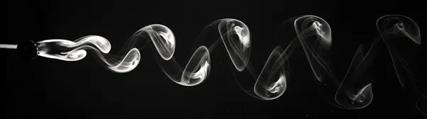
Kármán Vortex Street (or a von Kármán vortex street) is a repeating pattern of swirling vortices, caused by a process known as vortex shedding, which is responsible for the unsteady separation of flow of a fluid around blunt bodies

In fluid dynamics, vortex shedding is an oscillating flow that takes place when a fluid such as air or water flows past a bluff (as opposed to streamlined) body at certain velocities, depending on the size and shape of the body. In this flow, vortices are created at the back of the body and detach periodically from either side of the body forming a Von Kármán vortex street. The fluid flow past the object creates alternating low-pressure vortices on the downstream side of the object. The object will tend to move toward the low-pressure zone.

If the bluff structure is not mounted rigidly and the frequency of vortex shedding matches the resonance frequency of the structure, then the structure can begin to resonate, vibrating with harmonic oscillations driven by the energy of the flow. This vibration is the cause for overhead power line wires humming in the wind and for the fluttering of automobile whip radio antennas at some speeds. Tall chimneys constructed of thin-walled steel tubes can be sufficiently flexible that, in air flow with a speed in the critical range, vortex shedding can drive the chimney into violent oscillations that can damage or destroy the chimney

Reynolds number

The Reynolds number is defined as ratio of inertial forces to viscous forces within a fluid which is subjected to relative internal movement due to different fluid velocities

Where:

Re= (ρLu)/ (µ);

= (Lu)/ (ν)

ρ is the density of the fluid (SI units: kg/m3)

u is the flow speed (m/s)

L is a characteristic linear dimension (m) (see the below sections of this article for examples)

μ is the dynamic viscosity of the fluid (Pa·s or N·s/m2 or kg/(m·s))

ν is the kinematic viscosity of the fluid (m2/s).

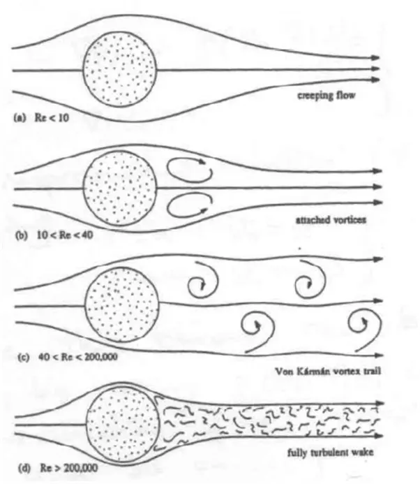
Flow characteristics flow over a cylinder for different Reynolds number

Steady state and transient state for re-100

Case (c) Re-100

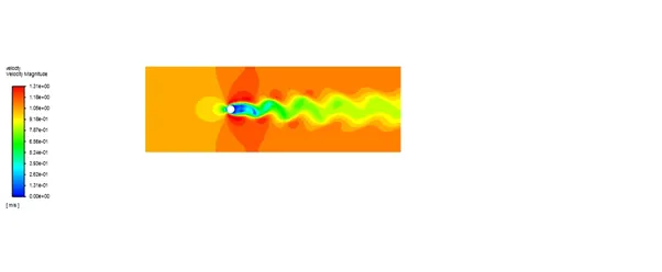
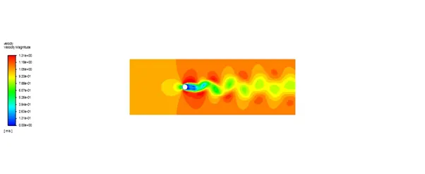
The flow over a cylinder in case(c) causes boundary separations and causing oscillating wakes at lower pressure side (right side in the fig c) these wiggles are named as Kármán Vortex Street

Setup:

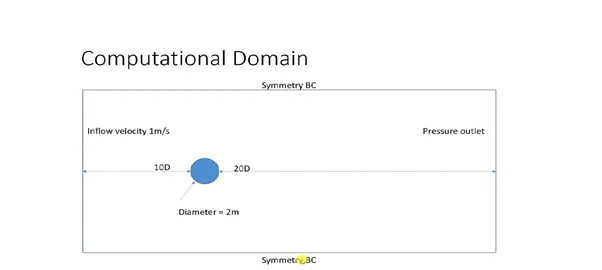
Creating this geometry in space claim

Meshing

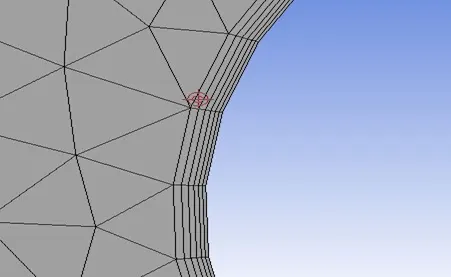
• Giving a finer mesh element to the geometry and selecting appropriate type of mesh element to get better physics
• Provide inflation layer on the cylinder to capture the wall boundary nicely

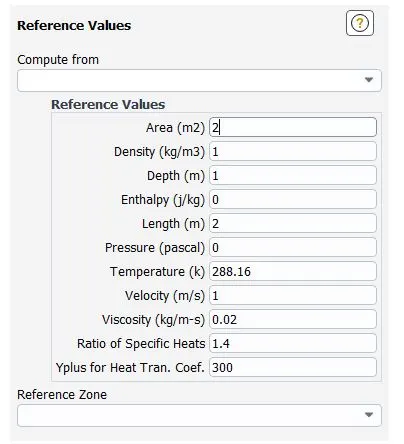
Reference values

It plays an important role in determining the plots

Area - it is used to determine co-efficient of drag and lift

The area of flow across top region of the cylinder looks like a rectangle with breadth as 2m that is dia of cylinder and thickness as 1, therefore area of the rectangle would be 2

1. Steady state and transient state (Case c)

Reynold number	100
Velocity	1m/s
Viscosity	0.02Pa-s

Results

Residual plots

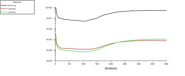
Steady state

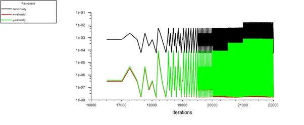
Transient state

Observations:

• In the case of steady state after 300 iterations we observe less fluctuation in the curve ,on this bases we consider that the flow as converged but other monitor points should be considered to assure that the flow as converged
• In the case of transient state convergence cannot be determined in this case for each time step is calculated unlike steady state (steady state are used to determine the end results giving less emphases on time state ),so we see other plots for convergence of results
• Transient case it takes longer time to converge than compared to steady state case

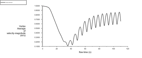
Monitoring the velocity at x-10, y-0

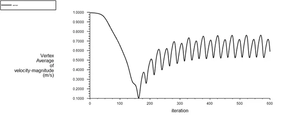
Steady-state

Transient state

Observations

• In steady state after 250 iterations we see similar types of resonance in the system showing convergence in the system
• In transient state after 70 time step we see similar type of resonance in the system

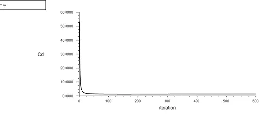
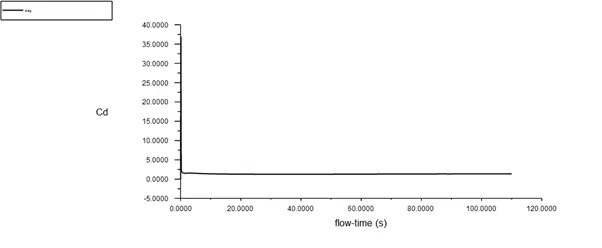
Co-efficient of drag

Steady-state

Transient state

Observations

• Both transient as well as steady state after zeroth time step there’s convergence in the result

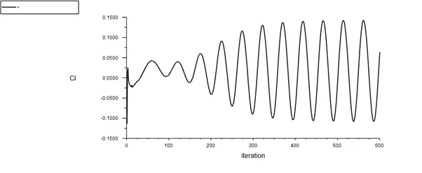
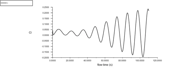
Co-efficient of lift

Steady-state

Transient state

Observations:

• In steady state case after 400 iterations we would see similar type of wiggles, therefore solution converges but transient case we needed run for few more time step for the convergence of the result

Velocity Contours

Steady state

Transient state

In transient state we can see more precise wiggles compared to steady state from the above contour plots

Conclusion:

In the residual plot in steady state case we observe no fluctuation in the system after some interval of iteration, the stability of the plot depends upon

• mesh type,
• mesh size
• Error of residual value

Less error of residual value leads more time to compute giving accurate results which are not always required, it also depends upon the object complexity through which the computation is done therefore choosing error of residual value for convergence should be normalised to compute the results faster and give accurate results

In transient case the residual plots we couldn’t estimate the convergence of the results (in steady state if the residuals doesn’t converge), so we look after other plots and monitor point plots

These plots (drag co-efficient, lift coefficient and monitor point velocity) all show similar kind of wiggles in the system so can conclude that the solution has converged

Strouhal number

The Strouhal number (St, or sometimes Sr to avoid the conflict with the Stanton number) is a dimensionless number describing oscillating flow mechanisms

The Strouhal number is often given as

St=fL/u;

Where f is the frequency of vortex shedding, L is the characteristic length (for example, hydraulic diameter or the air foil thickness) and U is the flow velocity

For large Strouhal numbers (order of 1), viscosity dominates fluid flow, resulting in a collective oscillating movement of the fluid "plug". For low Strouhal numbers (order of 10⁻⁴ and below), the high-speed, quasi-steady-state portion of the movement dominates the oscillation. Oscillation at intermediate Strouhal numbers is characterized by the build-up and rapidly subsequent shedding of vortices

For spheres in uniform flow in the Reynolds number range of 8×10² < Re < 2×10⁵ there co-exist two values of the Strouhal number. The lower frequency is attributed to the large-scale instability of the wake, is independent of the Reynolds number Re and is approximately equal to 0.2. The higher-frequency Strouhal number is caused by small-scale instabilities from the separation of the shear layer

1. Go to fluent solver > results >fft analyser>load lift co-efficient>select FFT plot
2. To get the magnitude of strouhal number,

Go to results > fft analyser > click on write fft to file >click on write fft

Open the file in excel and 1^st column denotes the frequency and 2^nd column denotes the strouhal number open the file in excel use maximum command in the second row to find the strouhal number

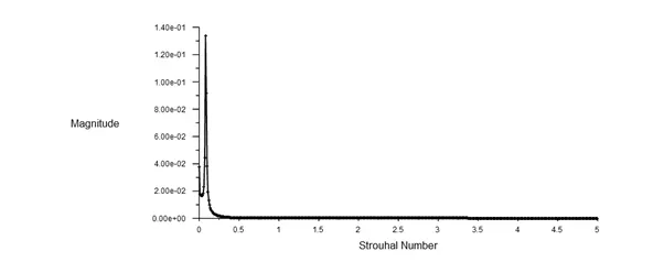
The strouhal number is found to be 1.34e-01

Observations

Results of Steady state for Reynolds no 10,1000,10000 and100000

Rey-10

Velocity	0.1m/s
Viscosity	0.02Pa-s

Residual plot

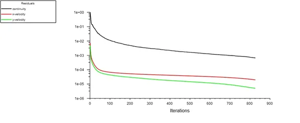
• After 800 iteration still the solution has not converged ,so we after other plots for convergence

Velocity monitor point

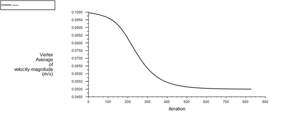
• After 600 iteration the solution has been converged

Drag co-efficient

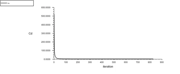
• After 100 iteration the solution will converge

Lift co-efficient

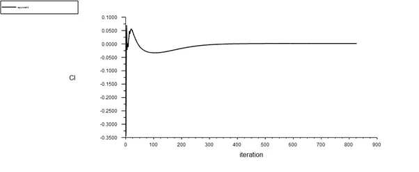
• After 400 iterations the solution converges

Velocity contour

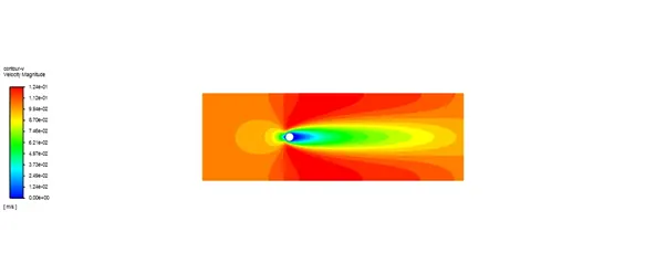
Rey-1000

Velocity	10m/s
Viscosity	0.02Pa-s

Residual plot

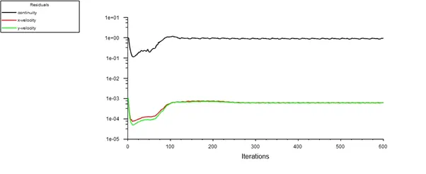
• After 200 iteration the solution converges

Velocity monitor point

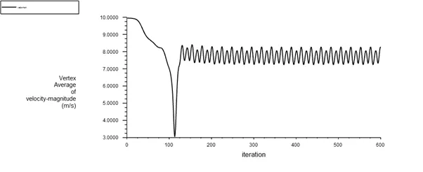
• After 200 iterations similar kind of wiggles are formed

Drag co-efficient

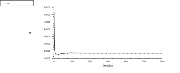
• After 100 iterations the solution converges with minor fluctuation

Lift co-efficient

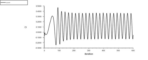
• After 150 iteration similar kind of wiggles are formed ,the solution converges

Velocity contour

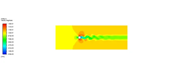
Rey-10000

Velocity	100m/s
Viscosity	0.02Pa-s

Residual plots

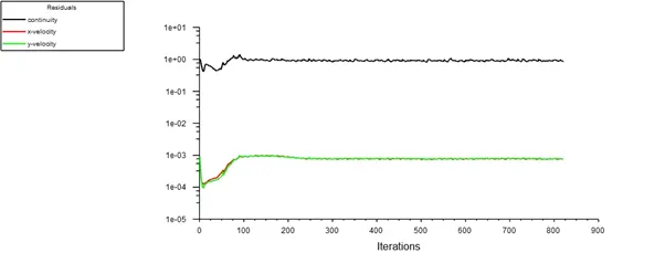
• After 200 iteration the solution converges with minor negligible fluctuation in the system

Velocity monitor point

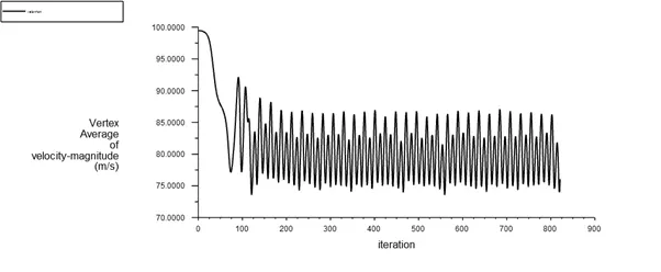
• After 200 iteration the solution converges with similar wiggles in the system

Drag co-efficient

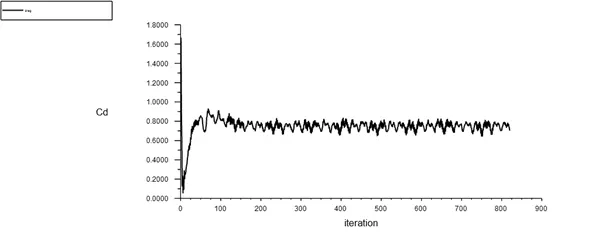
• After 200 iteration the solution converges with similar wiggles in the system

Lift co-efficient

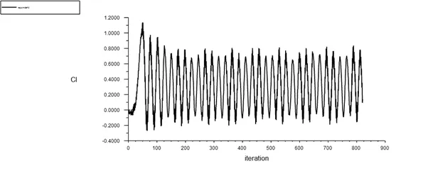
• After 200 iteration the solution converges with similar wiggles in the system

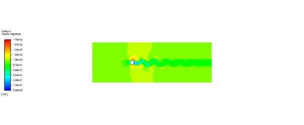
Velocity contour

Rey-100000

Velocity	1000m/s
Viscosity	0.02Pa-s

Residual plots

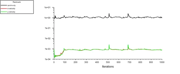
• After 800 iteration still the solution has converged with less fluctuation in the system

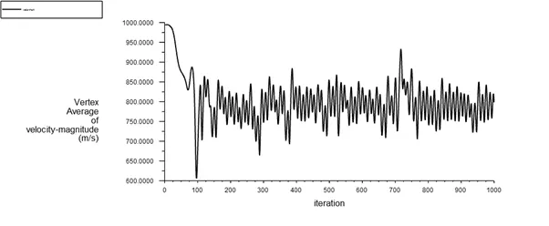
Velocity monitor point

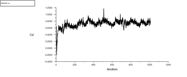
Drag co-efficient

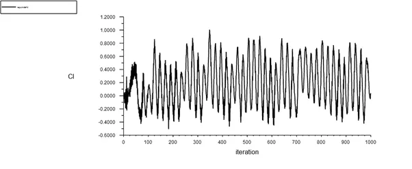
Lift co-efficient

Observations

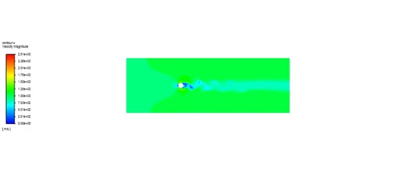
From the above plot we can see that solution as not converged the flow has become turbulent that it has hard to find similar wiggles in the system snce flow of the flud has turned turbulet

Contour plot-velocity

Effect of Reynolds number on co-efficient of drag and lift

Reynolds number	Co-efficient of drag	Lift co efficient
10	3.323	0.0015
100 steady	1.333	0.033
1000	0.716	0.125
10000	0.702	0.339
100000	0.691	0.195

Conclusion

For different Reynold number cases we find that lift and drag co-efficient are calculated after 10,000 the Reynold number are more turbulent the co-efficient of drag decreases this because flow attachment to body of the cylinder would me more compared to that of laminar flow (i.e. flow separation for turbulent layer at far distance compared to laminar flow) there would be larger mixing in the fluid layers