Week 2 - Flow over a Cylinder.
Aim:
The objective of the project is to simulate the flow over the cylinder for the steady state & unsteady state conditions. The simulation will be carried out for various Reynolds number. The simulation will be carried out in the Ansys Fluent workbench. For the first part, simulation for Re 100 in steady & unsteady conditions & strouhal number need to be calculated for Re 100. For the second part of the challenge is to calculate drag & lift coefficient for the flow over a cylinder for the series of Reynolds Number, 10, 100, 1000, 10000, & 100000. The steady state simulation has been used for the second part.
Introduction:
The simulation of flow over the cylinder is very challenging for the reseracher till today. This simulation is very useful to understand the complex behavious of fluid mechanics. Some of the applications are to understand the unsteady dynamics of wake flow behind the cylinder, cross flow normal to the stationary cylinder & the problems related to the mass & heat transportations. This problems are related to wide variety of problems faed by the engineering field.
The two most important phenomena associated with this type of simulations are vortex shedding & kamran vortex street.
Vortex Shedding:
It is a phenomena when the flow crosses the bluff body, vortices are shed alternately from one side to the other, & where alternating low-pressure zones are generated to the downside of the bluff body giving rise to a fluctuating force acting at right angles to the flow direction.
Von Kamran Vortex Street:
The vortices which are sheded alternately from either side of the bluff body & it creates the pattern of swirling vortices. These pattern of swirling vortices are repeated periodically & its called as von kamran vortex street.
Depends on the force, the body might move towards the direction of the force. If the bluff body doesnt mounted rigidly on the structure than it will start vibrating with harmonic oscillations driven by the energy of the flow & if the vortex shedding frequency of the vibration reaches the frequency of the structural-vibration frequency of the body than the body start resonating. This phenomenon is of major importance in engineering design because the alternate formation and shedding of vortices also creates alternating forces, which occur more frequently as the velocity of the flow increases.
When the frequency is in the audible range, a sound can be heard and the body appears to sing. Many structures failed because of this phenomena. Because of this effect, it is very important to study the vortex sheding to make sure performance of the components will not affect by the vortex shedding. The strouhal number has been used while studying this type of phenimena.
Strouhal Number (Sr or St):
This is a dimensionless number which used to to a measure of the vortex shedding frequency. This number is function of Reynolds number but less of surface roughness & freestream turbulence.
Design Inputs:
Material: Air
Density: 1 kg/m^3
Viscosity: 0.02 NS/m^2
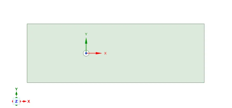
The model has been created into the Spaceclaim.
Dimensions:
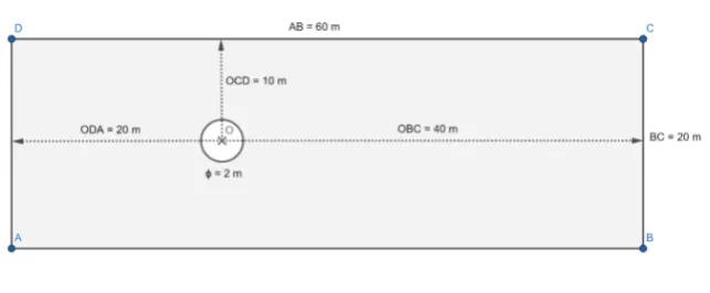
Model:
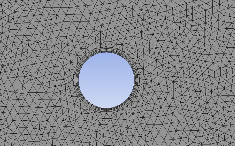
Meshing:
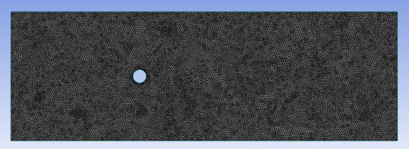
Mesh element size: 0.25m
Method: All Triangles
Edge Sizing: (Around Cylinder): 36 Number of divisions
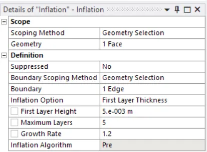
Infaltion Layers:
Mesh Quality:
Named Selection:
Simulation setup:
For Steady State:
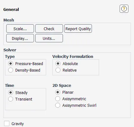
For unsteady, the Transient option has been selected instead of steady.
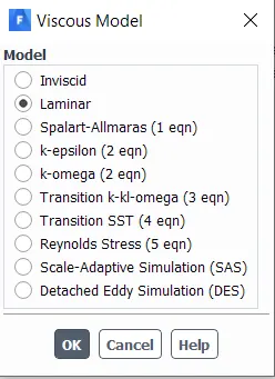
Viscous Model:
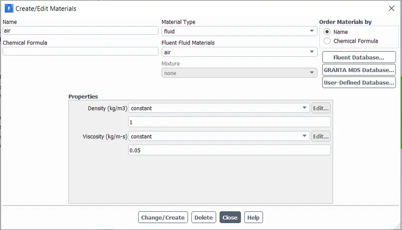
Material:
Re 100 has been set using the viscosity of the material as we can not enter Reynolds number directly into the fluent software.
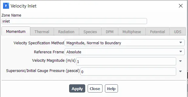
Boundary Conditions:
For Inlet
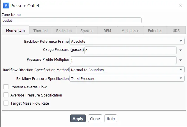
For Outlet
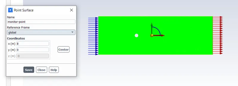
Created Monitor Point to measure velocity profile at that point.
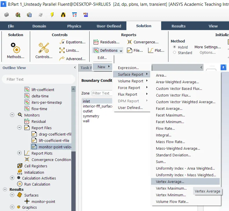
The surface report has been created using the Vertex Average option to monitor the velocity changes with each iteration at monitor point.
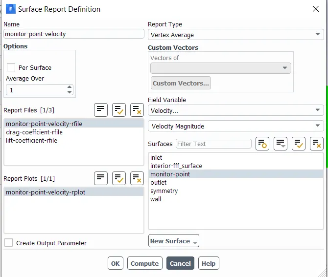
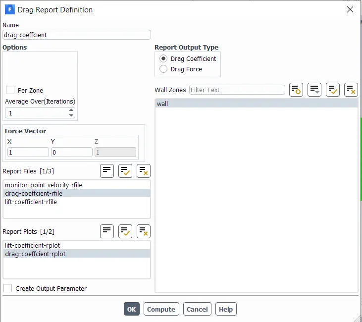
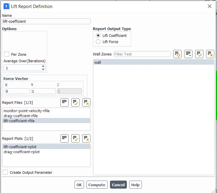
Surface report to measure velocity at the monitor point, drag coefficient & lift coeffcient has been created to record the values for each iteration.
Monitor point velocity
Drag Coeffcient
Lift Coefficient
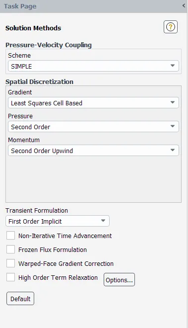
Solution Method
Velocity contour & pressure contour graph has been created from the Results> Graphics.
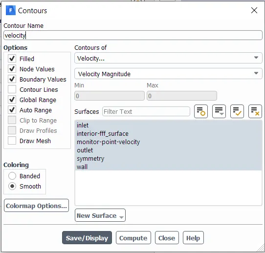
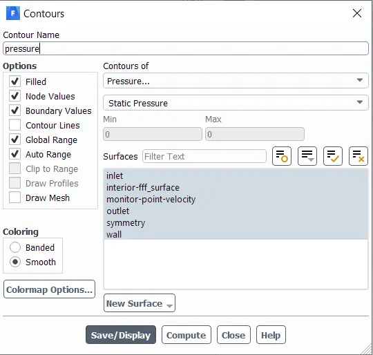
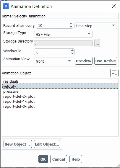
Animation of velocity contour graph has been created to visualize the wake field generated behind the cylinder & also vortex shedding phenomena.
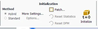
Initializing simulation
Following are the images of the post processing of Part 1 of the chalenge.
Part 1:
In this part results for, for Re 100, steady & unsteady simulation will be presented.
For Steady & Unsteady State simulation:
Viscosity: 0.02 kg/m^3
Flow Velocity: 1 m/s
Calculating Strouhal Number for Re 100:
For 40<Re<150, the Strouhal Number is
`Sr ~~ 0.198 (1 - 19.7/(Re))`
So, Sr = 0.16 for Re 100.
Procedure to create Strouhal Number in Fluent:
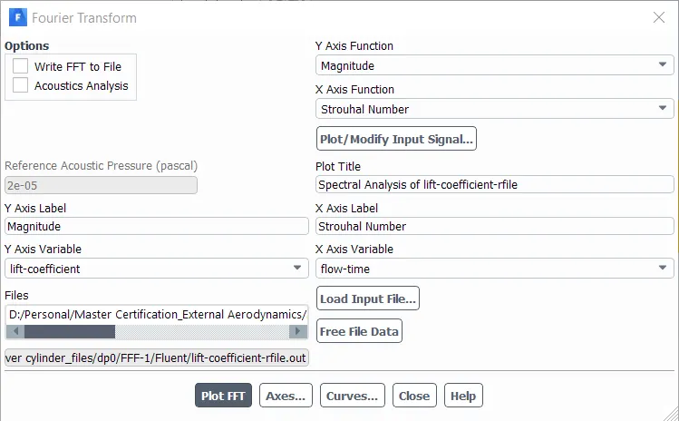
The FFT plot has been used to plot Strouhal Number. The lift coefficient data has been given as an input. The magniture option has been selected from drop down menu for Y-axis & Strouhal number for x-axis. The strouhal number plot has been displayed with the results images of each simulation.
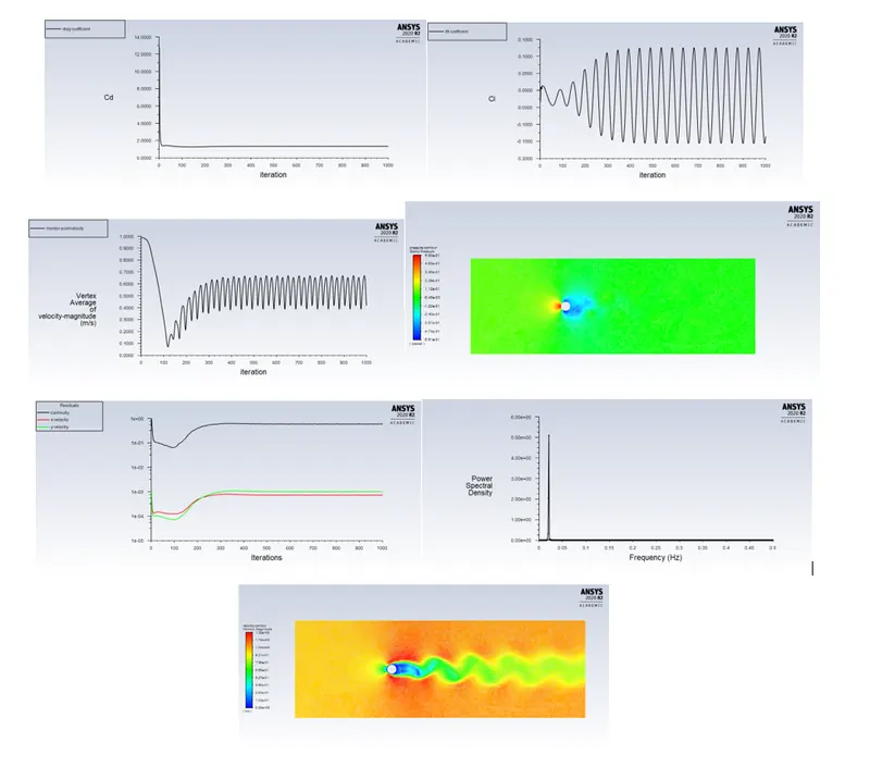
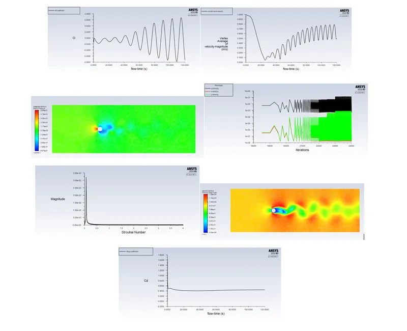
The images has been presented for drag coefficient, lift coefficient, monitor pint velocity, pressure contour, residuals, strouhal number & velocity contour.
Results for Steady State Simulation
Animation to Visualize vortex shedding phenomena
Results For Unsteady State Simulation
Animation:
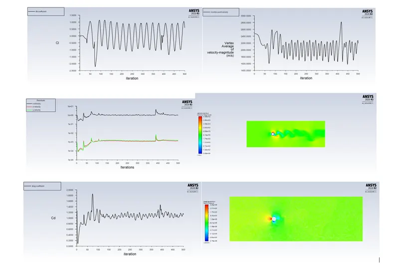
From above images following observations can be made.
1. In residual plot, the error value is neither changing not increasing from the set limit of 1e-3, that's why it can be said that the solution is converged.
2. In velocity contour plot, the von kamran vortex street can be seen, but it can be seen properly in the below animation file.
3. In pressure contour image, the low pressure field is changling alternately. It can be seen by observing the blue area. The low pressure wake field is the primary physics to observe for this challenge.
4. In lift coefficient plot, the vaue is kept rising & faling because of vortex shedding phenomena. The lift coefficient data has been used in the Fourier Transform (FFT) plot to plot the strouhal number.
5. The drag coefficient value is constant after one point. The drag coefficient of the cylinder is calucalated by the fluent is around 1.33.
The drag coefficient values has been compared with the experimental data provided in the following research paper written by B.N. Rajani which is "Numerical simulation of laminar flow past a circular cylinder". The drag coefficient values are within the 5% variance in comparison with the experimental data.
Similar observations can be made for all graphs presented for each simulations carried out.
6. The strouhal number determined by taking the median of the plot data in the Fluent software is 0.25 for both steady & unsteady state simulation. Through analytical method, the strouhal number is calculated as 0.16. So, the strouhal number of fluent is nearer to the analytical method.
Part 2:
Flow velocity has been used for each simulation as per following table according to the Reynolds Number, Density & viscosity. The steady state solver has been used for all simulations. The simulation results for Re 100 has been displayed in Part 1.
The material density, characteristic length & dynamics viscosity has been shown in the below table with the Reynolds number with their respective flow velocity calculated uisng the Reynilds number equation.
The equation of Reynolds number is
`Re = (rho* U * L)/mu`
where,
Re = Reynolds number
`rho` = material density
U = flow velocity
L = characteristic length
`mu` = dynamic viscosity
| Density | 1 | kg/m^3 |
| Characteristic Length | 2 | m |
| Dynamic Viscosity | 0.05 | kg/m/s |
| Reynolds Number | Flow Velocity | Unit |
| 10 | 0.25 | m/s |
| 100 | 2.5 | m/s |
| 1000 | 25 | m/s |
| 10000 | 250 | m/s |
| 100000 | 2500 | m/s |
The model generation using spacclaim & simulation setup has been carried out in a similar way as explained before. The post processing images has been presented for each simulation.
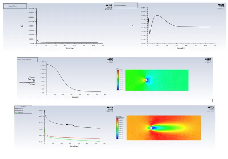
For Re 10:
Animation:
The animation & the velocity contour shows that the vortex shedding is missing for the Re 10. The reason behind this is that vortex shedding doesnt occur below 40.
For Re 100:
Results were shown in part 1.
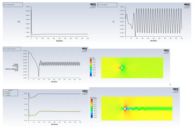
For Re 1000:
Animation:
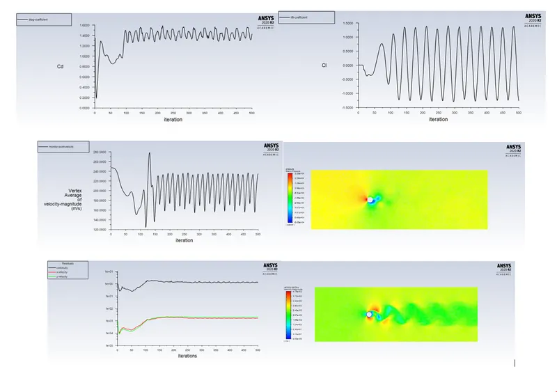
For Re 10000
Animation:
For Re 100000:
Animation:
Discussion & Conclusion:
The time & resources consumes by the transient solver is far more than the steady state solver.
For the transient simuations, the simualtion were running after turining off the convergence criteria. In transient mode, the more iterations are required to develop proper physics of the flow. Because of that the transient simuation has taken more iteration with smaller time steps compare to the steady state.
The drag coefficient for the Re above 1000, is start fluctuating but periodic after one point which can be seen from the results images. So statistically, it is constant.
The results of the simulations are the one we are expecting from the physics point of view.
The challenge of simualting flow over a cylinder has been carried out to study the vortex shedding phenomena & visualizing von kamran vortex street. The challenge has been divided into two parts. In first part, the steady& unsteady state simulations have been performed for Re 100 & strouhal number has been calculated using analytical method & later compared with the fluent result. While in second part series of simualtion has been carried out for various Re numbers in steady state consition. Vortex shedding & kamran vortex street was unable to visualize for Re 10 because these two phenomena doesnt occur below Re 40. The drag coefficient & lift coefficient has been compare for all simulations.
References:
1. https://thermopedia.com/content/1247/
2. https://www.sciencedirect.com/topics/engineering/vortex-shedding
3. Research Paper writtin by B N Rajani called "Numerical simulation of laminar flow past a circular cylinder".