Week 2 - Flow over a Cylinder.
AIM:
To simulate the flow over a cylinder and explain the phenomenon of Karman vortex street.
INTRODUCTION:
- There are two main types of drag:
- pressure drag, which is dominant in blunt bodies due to flow separation and the formation of a wake,
- friction drag, which is significant in streamlined bodies due to wall shear stress.
- At higher Reynolds numbers, blunt bodies can experience vortex shedding, which leads to vibration and noise.
- However, a turbulent boundary layer helps delay separation, reducing the size of the wake and pressure drag.
- In contrast, streamlined bodies are designed to minimize separation, making friction drag the dominant factor.
- Engineers aim to maintain laminar flow to minimize friction drag, but sometimes turbulent flow is introduced intentionally to prevent flow separation and reduce overall drag.
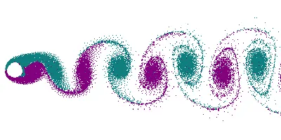
VORTEX SHEDDING is an oscillating flow that takes place when a fluid such as air or water flows past a bluff (as opposed to streamline) body at certain velocities, depending on the size and shape of the body.
It happens because of flow separation and pressure difference on either side of the object.
Example:
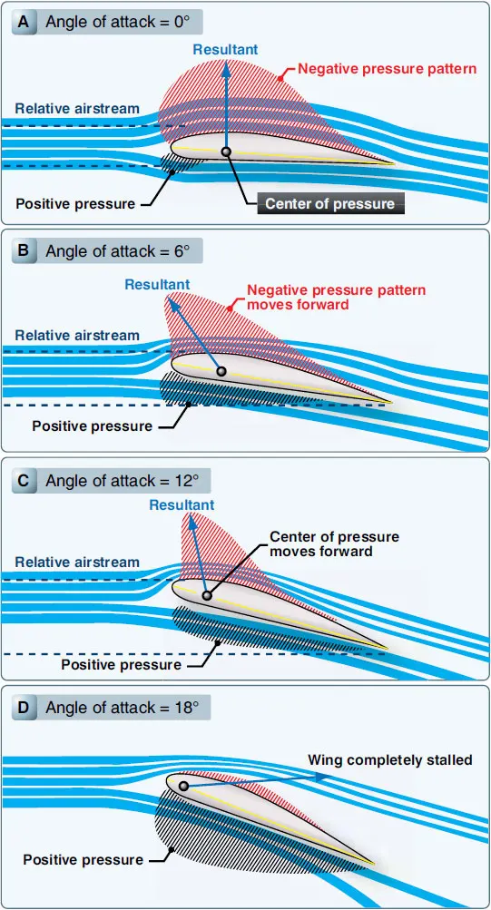
- In aero wings, airfoils are shaped to create the pressure difference whereas, high pressure is below surface, and low pressure is above surface.
- the pressure difference generate lift which helps the aero place rise and stay in the air.
- In case of airfoils, why there is vortex shedding is because airfoils have smooth streamlined shapes that helps maintain attached flow, minimizing separating and thus avoiding vortex shedding under normal condition.
- if the angle of attack is increased, we can experience the vortex shedding in aero plane too.
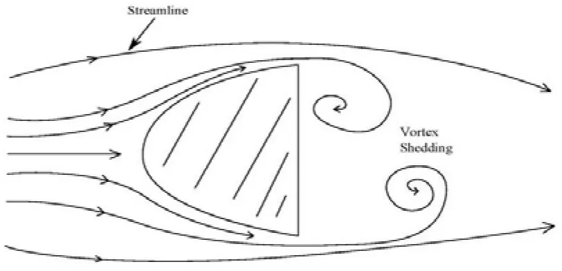
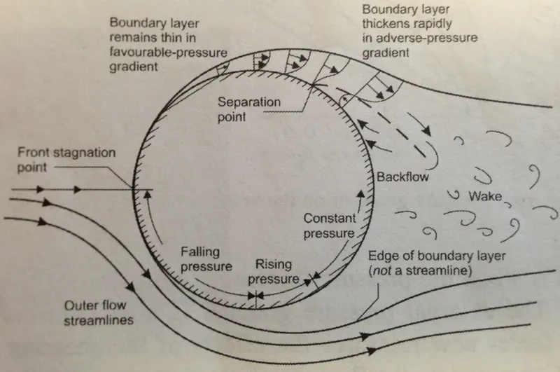
- But in the case of bluff body, due to their shape, the boundary layer separates early on both sides, creating a large wake region.
- the flow is this wake becomes unstable and starts shedding vortices alternately which is known as vortex shedding.
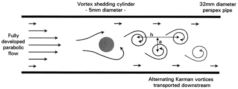
KARMAN VORTEX is a repeating pattern of swirling vortices, caused by process known as vortex shedding, which responsible for unsteady separation of flow of flid around blunt bodies.
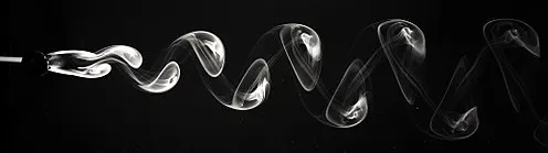
so, Vortex shedding is the process and Karman vortex is the outcome / pattern
Is vortex shedding is good or bad
It can be both good and bad- depending on the situation.
when vortex shedding is good
- cooling and mixing application
- vortex lift
when vortex shedding is bad
- structural vibration/resonance
- noise and vibration
- instability in flight
How to quantify vortex shedding
The most important formula is based on the Strouhal number (St)
St = (f x D) /u
where,
St - Strouhal number (dimensionless)
f - vortex shedding frequency (Hz)
D - characteristic length (m) - like diameter of cylinder
U - free stream velocity (m/s)
Relationship between Strouhal number and Reynolds number:
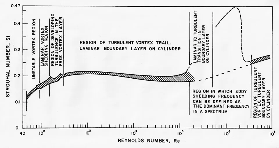
the above graph represents of how vortex shedding frequency and flow regimes changes with varying Reynolds number
Unstable vortex region (Re: 40 - 100)
- flow is creeping and no periodic vortex shedding occurs
- vortices may form randomly, not in an organized fashion
- Strouhal number is undefined or very low
Laminar vortex shedding (Re: 100 - 300)
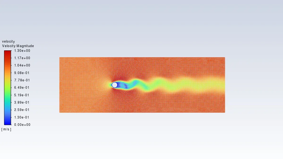
- vortices begin shedding alternatively from top and bottom (Karman vortex street begins)
- alternating vortices shed in a predictable pattern
- the cylinder boundary layer is laminar, and the wake is smooth
Region of developing turbulence in the free vortex tube (Re: 300 - 750)
- the free shear layers (rolled up vortices) become turbulent, but the boundary layer on the cylinder stays laminar
- vortex shedding remains periodic but less regular.
Turbulent vortex trail (Re: 750- 10,000)
- the wake is fully turbulent, but the cylinders boundary layer remains laminar
- vortex shedding is still detectable but obscured by small scale turbulence
- this is the typical vortex shedding region used for engineering applications
- This is the region where CFD and experiments give reliable frequency results
Transition zone (Re: 10,000- 100,000)
- boundary layer on the cylinder transition to turbulent
- Strouhal number behavior becomes irregular - shown by dotted lines and jumped behavior
- flow separation moves backward on the surface due to turbulent boundary layer.
Fully turbulent boundary layer (Re > 10,00,000)
- The boundary layer on the cylinder becomes turbulent
- Strouhal number stabilizes again
- vortex shedding continues but the shedding pattern and separation point differ.
GEOMETRY CREATION: (space claim)
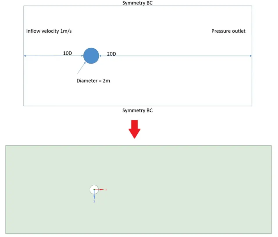
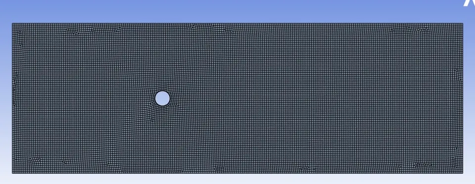
geometry is created as below model diagram. the length will be 60 m, and width will be 20 m.
MESHING:
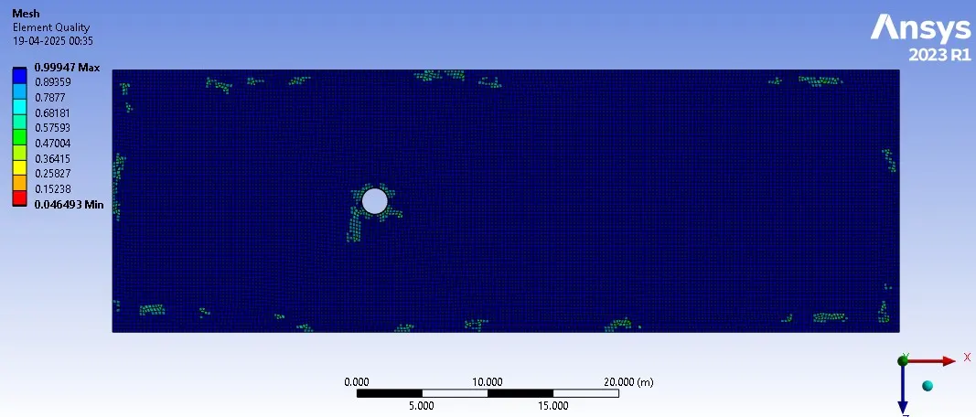
The mesh used here is 2D hexa mesh, to attain unform layer throughout the surface.
the mesh size is kept is 0.25 m which is finer mesh for this model
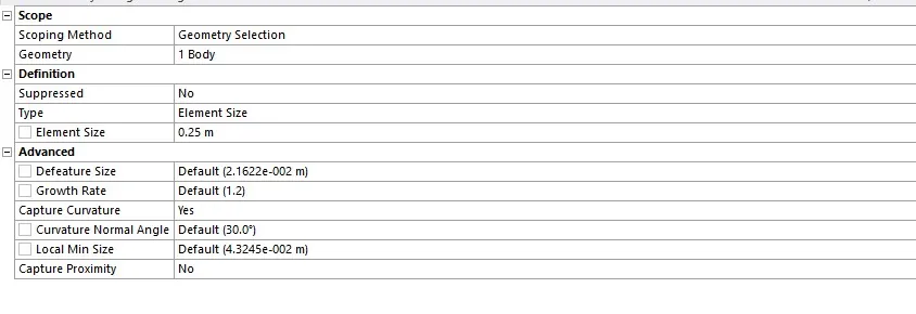
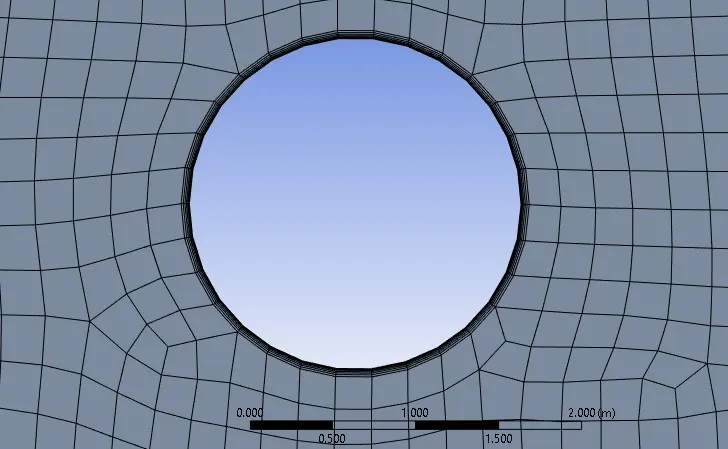
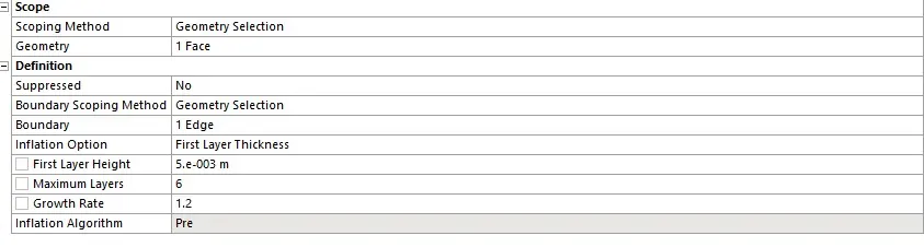
In cylinder area, it has been much refined by using inflation option which gives the layer of mesh around the cylinder (6 layers - 0.003 m) with growth rate of 1.2
the overall mesh element will be 19370 and nodes is 19696 which is almost (1:1)

the element quality also much good as we can see, most of the elements are fall more than 0.9 range (where mesh quality of 1 - sign of good mesh, and mesh quality of 0 - sign of bad mesh)
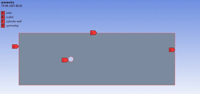
Named selection is provided for the important parameters for this problem. this will help to read fluent automatically to set the boundary condition using the named selection.
FLUENT - STEADY STATE (Setup):
- Viscous option is kept as Laminar, as we need to capture the vortex shedding (when we switched to turbulent vortex shedding will be there but also high discontinuity. this is the real-world application)
- Solver type - pressure based solver as we are solving for incompressible fluid
- velocity formulation - absolute as the model is considered as the stationary reference
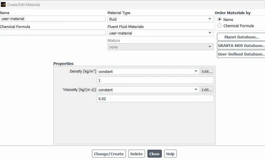
- create a new material, as the density of the material will be 1 kg/m3 and viscosity will 0.02 kg/ ms.
- the reason for new material is because, to make life easier we are going with simple values for academic calculation
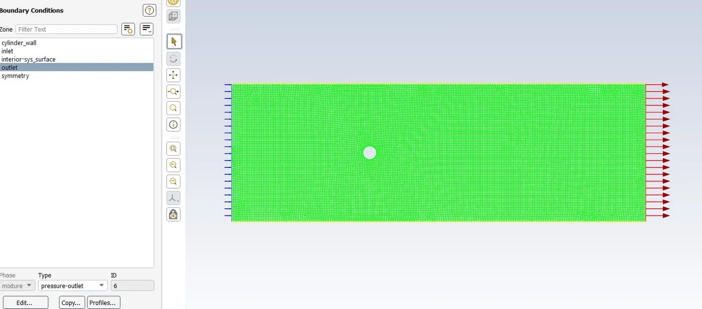
- the velocity of the inlet in this problem is depends on the Re value as shown in the below solution setup.
- as we discussed previously the boundary condition of the problem is attained automatically using the named selection which we have given.
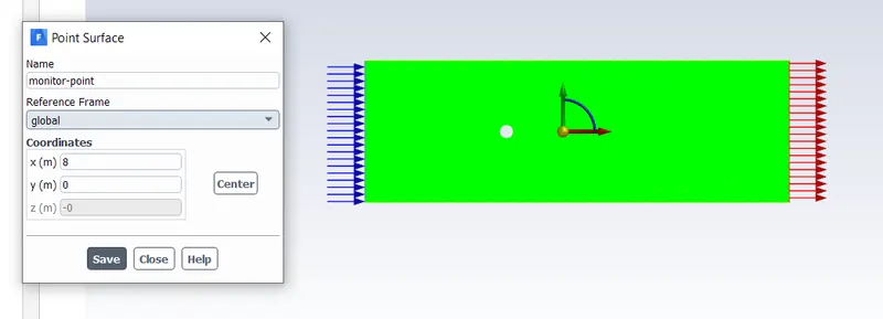
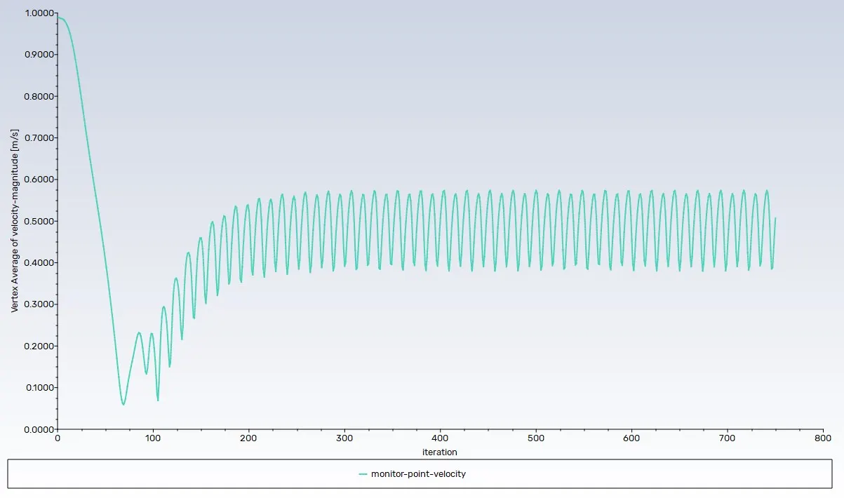
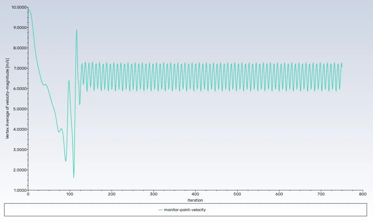
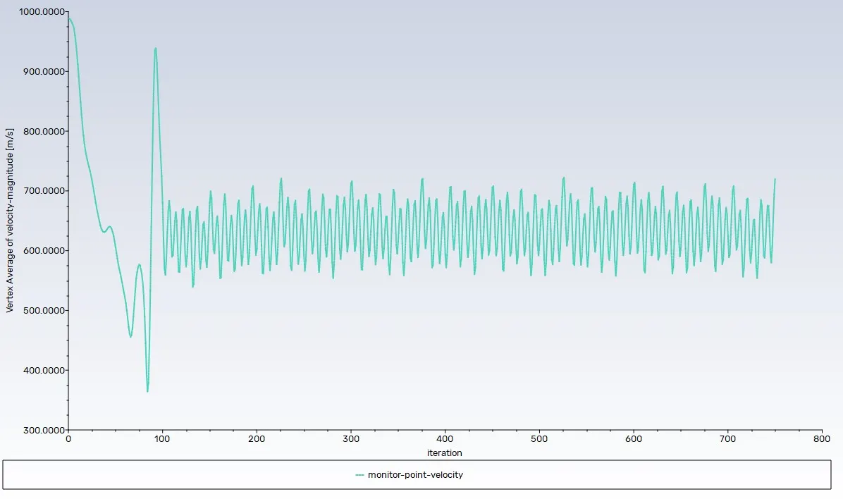
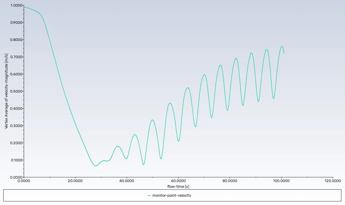
- the monitor point is created to observer the change in that particular location.
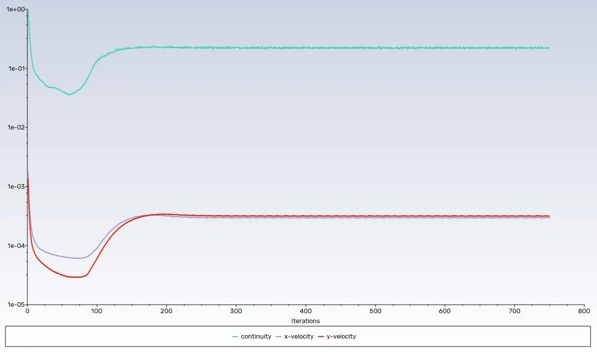
- In residual graph, the drag co-efficient, lift co-efficient, scaled residual, monitor point velocity graph are captured.
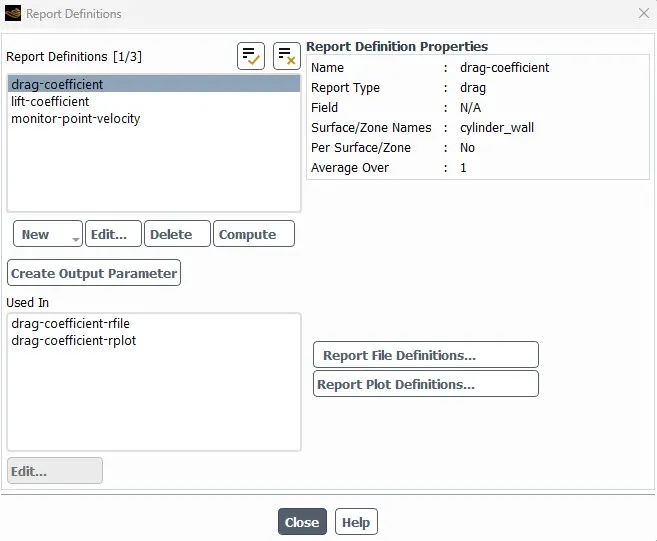
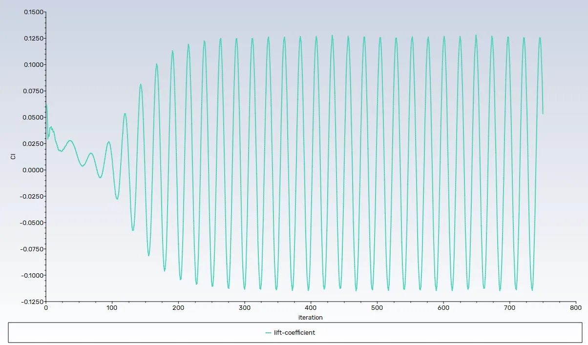
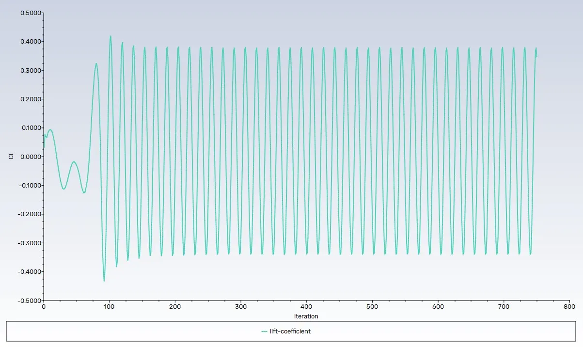
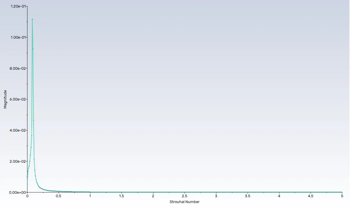
- from this data point of lift co-efficient we can calculate the Strouhal number
- where Strouhal number (St) is a dimensionless number that describes oscillation flow mechanism especially in vortex shedding
St = (f * L) / U
where,
f is the vortex shedding frequency (Hz)
L is the characteristic length (typically diameter of a cylinder, m)
U is the free stream velocity (m/s)
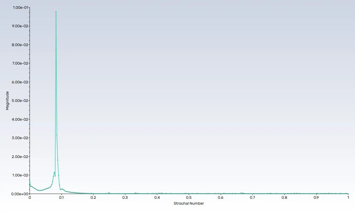
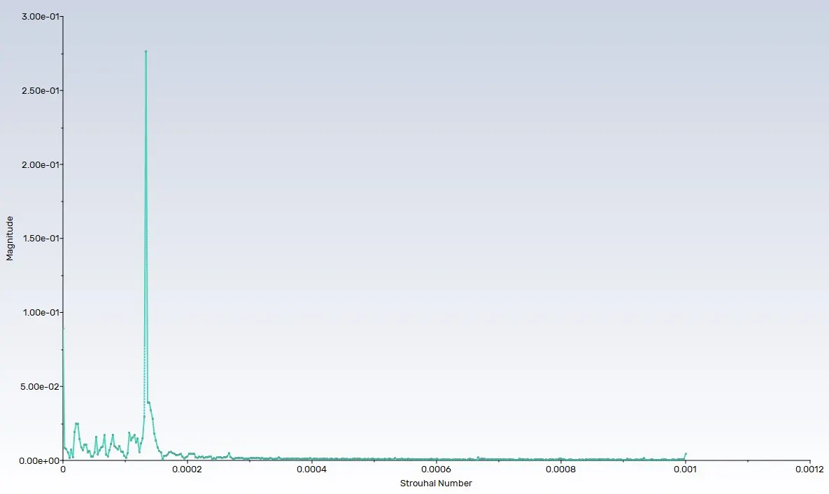
- the frequency is calculated by FFT method in Ansys fluent
- FFT converts data points which are typically function of time into frequency.
- so, if we have data collected over time (iteration) like lift co-efficient CL FFT reveals the dominant frequencies that Govens the oscillation in the signal.
- the reason we are using lift force co-efficient for Strouhal number is because lift is generally more sensitive to instabilities caused by vortex shedding especially flow around bluff bodies.
- while subsituting in above formula we will get the Strouhal number.
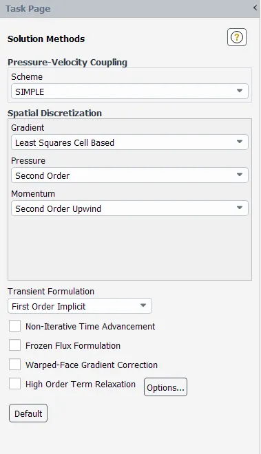
- the solution method is used here is simple.
- Velocity contour & pressure contour graph has been created from the Results> Graphics.
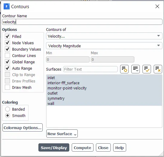
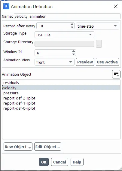
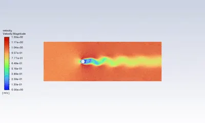
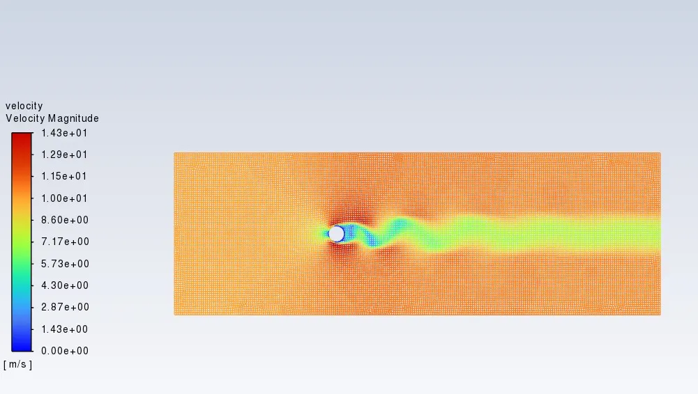
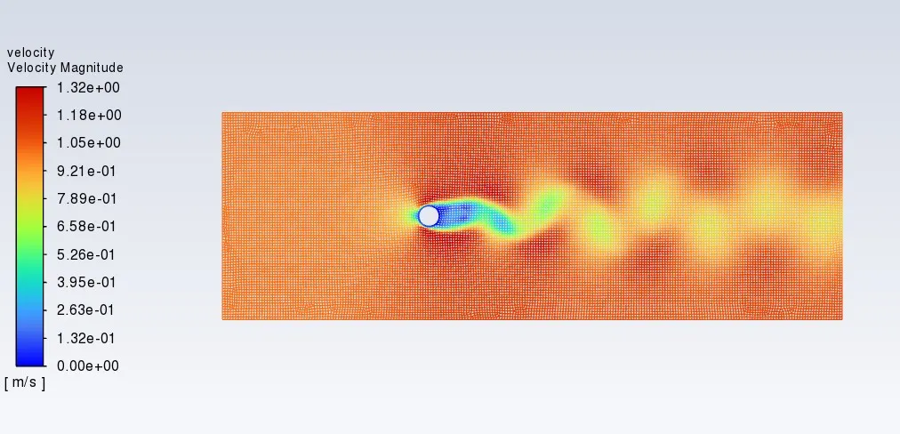
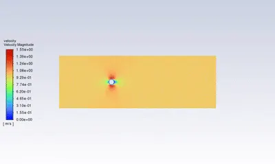
- Animation of velocity contour graph has been created to visualize the wake field generated behind the cylinder & also vortex shedding phenomena.
- then the solution has been initialized
Configuration 1: (Re = 10)
We know that Reynold number:
Re = (ρ * V * D) / μ
Where,
ρ - density of the fluid
V - velocity of the fluid
D - diameter of the cylinder
μ - absolute viscosity of the fluid
for the data the equation will be,
10 = (1 * V * 2) / 0.02
V = 0.1 m/s
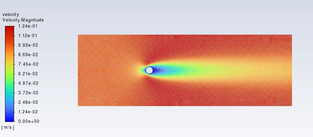
Velocity magnitude:
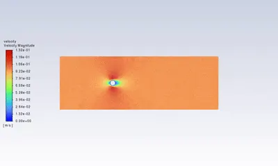
- the flow separates but remains steady and symmetric - no vortex shedding
Vertex average velocity at monitor point:
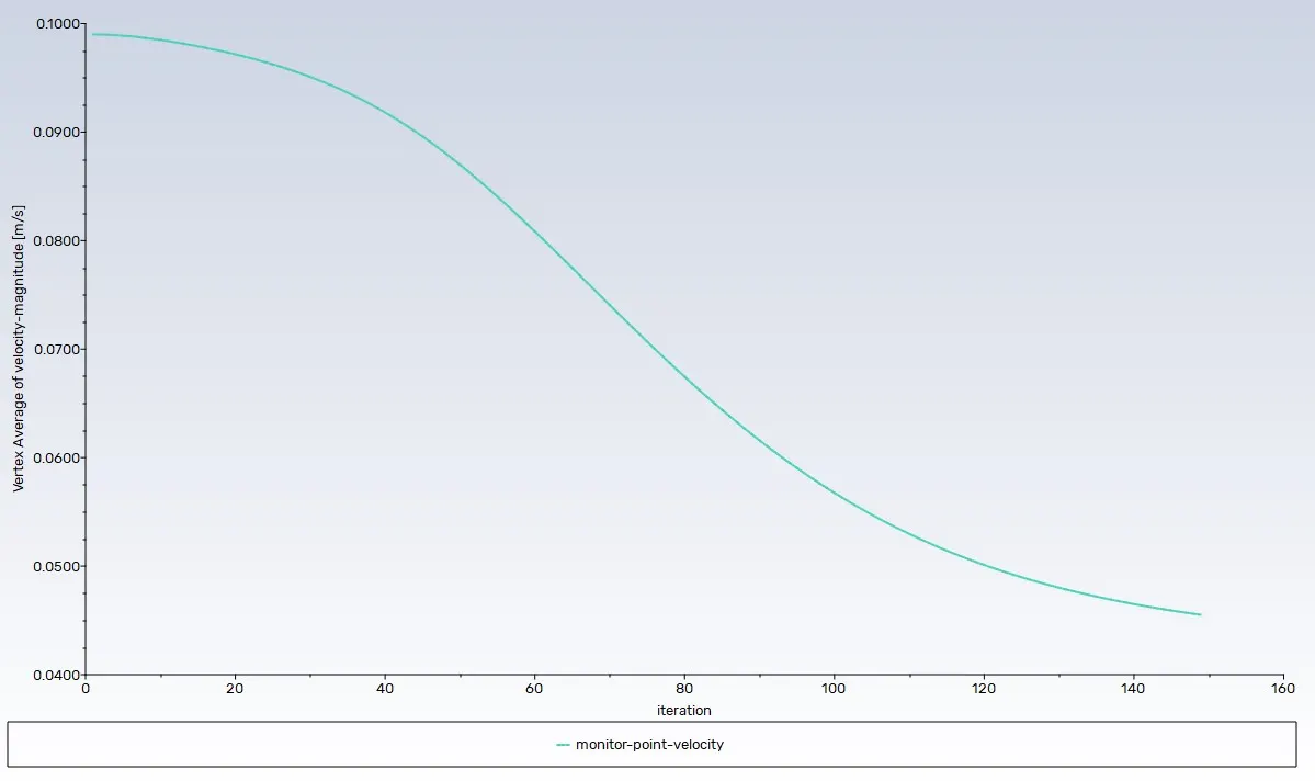
- the vertex average velocity graph shows how the residual or maximum velocity magnitude evolve with each iteration.
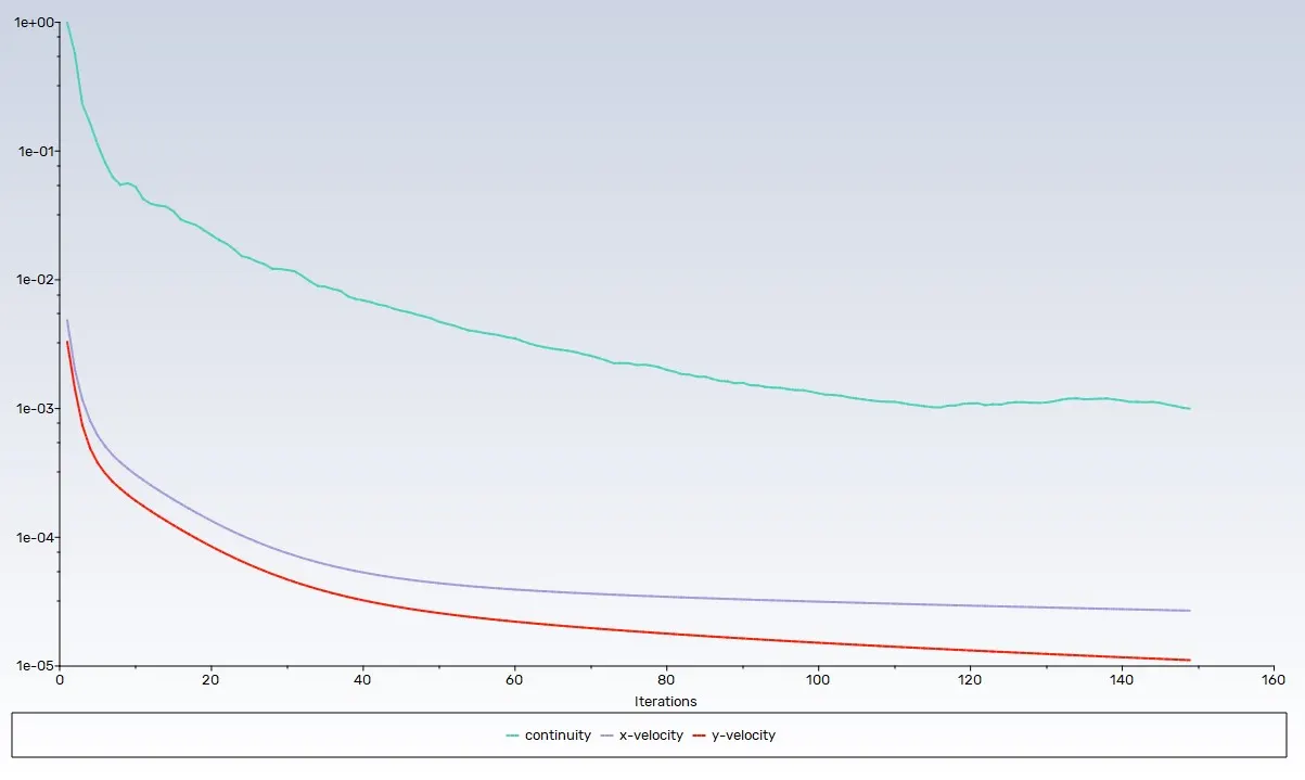
- as there is no vertex shedding in this Re, we can see that the magnitude of the velocity is very much smaller and decreasing logarithmically.
Scaled residual:
- the residual of all the points is dropping rapidly and reached the convergence criteria of 0.0001
Lift co-efficient:
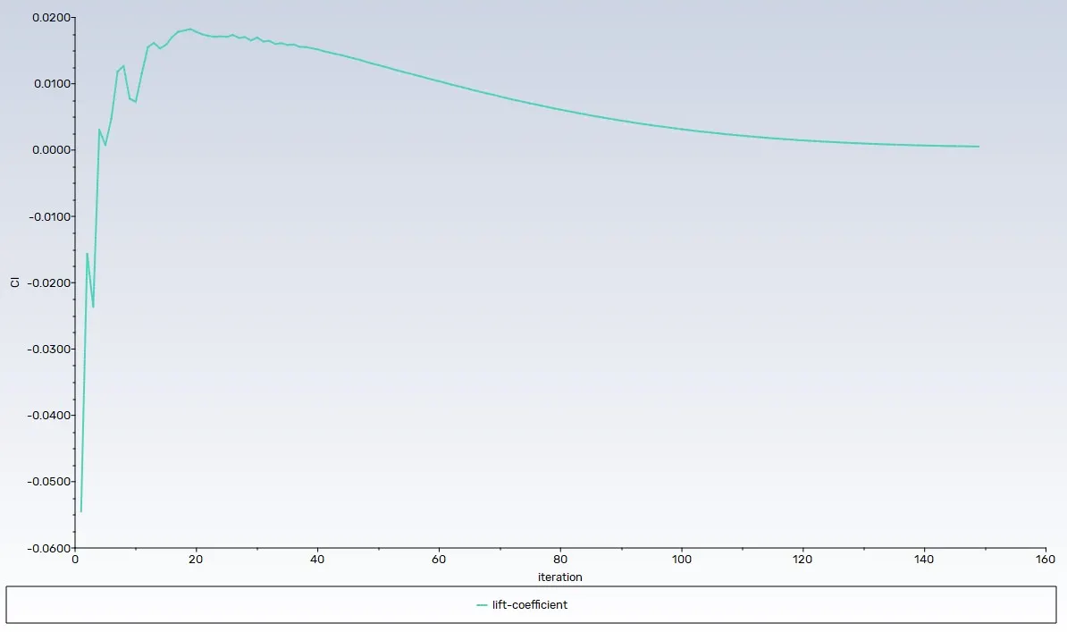
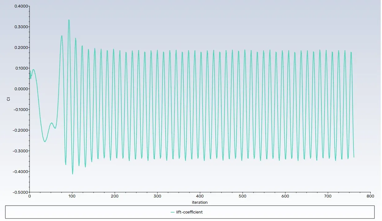
- the lift co-efficient will helps to study the Strouhal number, this is because vortex shedding generates an oscillating lift force, and the frequency of that oscillation is used to calculate the Strouhal Number.
- From the graph, it can be justified that after 200 iterations, the lift coefficient stabilizes around zero.
- This indicates that no vortex shedding has occurred, and the flow has reached a steady, symmetric state, which is typical for Reynolds numbers below ~47
Drag co-efficient:
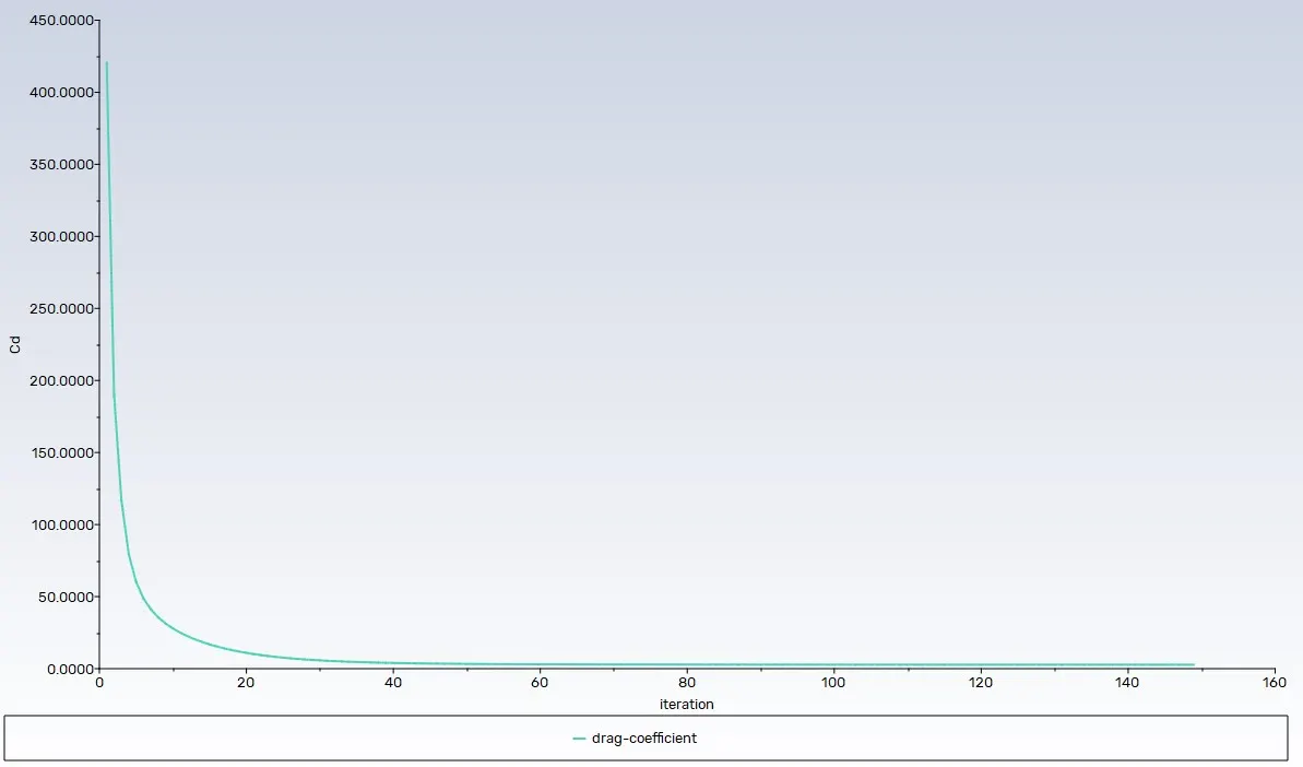
the drag force value drops to almost 0.08. this is because as there is no vortex shedding occured.
Convergence rate for X-velocity, Y-velocity and momentum:
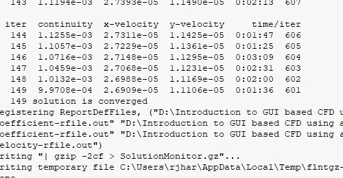
with Re - 10, the solution residuals have converged in 503 iterations for steady state.
Strouhal number:
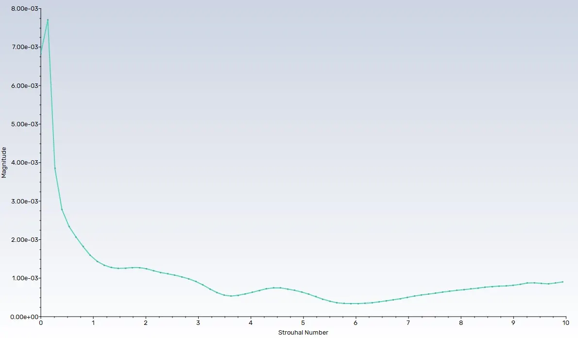
- so, as we discussed before the lift coefficient is monitored, and the graph is shown above with respect to no. of iteration
- with the help of fast fourier transform (FFT), the lift co-efficient is converted to frequency domain
- then it is used the compute the strouhal number with the help of the above strouhal formula as discussed.
Animation:
REPEAT THE PROBLEM AS DISCUSSED ABOVE BUT WITH DIFFERENT Re, TO QUANTIFY THE EFFECT OF RE FOR VORTEX SHEDDING.
Configuration 2: (Re = 100)
We know that Reynold number:
Re = (ρ * V * D) / μ
Where,
ρ - density of the fluid
V - velocity of the fluid
D - diameter of the cylinder
μ - absolute viscosity of the fluid
for the data the equation will be,
100 = (1 * V * 2) / 0.02
V = 1 m/s
Velocity magnitude:
Vertex average velocity at monitor point:
Scaled residual:
Lift co-efficient:
Drag co-efficient:
Convergence rate for X-velocity, Y-velocity and momentum:
Strouhal number:
Animation:
Configuration 3: (Re = 1000)
We know that Reynold number:
Re = (ρ * V * D) / μ
Where,
ρ - density of the fluid
V - velocity of the fluid
D - diameter of the cylinder
μ - absolute viscosity of the fluid
for the data the equation will be,
1000 = (1 * V * 2) / 0.02
V = 10 m/s
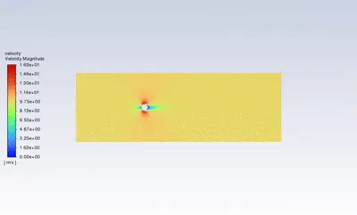
Velocity magnitude:
Vertex average velocity at monitor point:
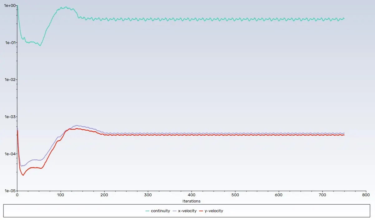
Scaled residual:
Lift co-efficient:
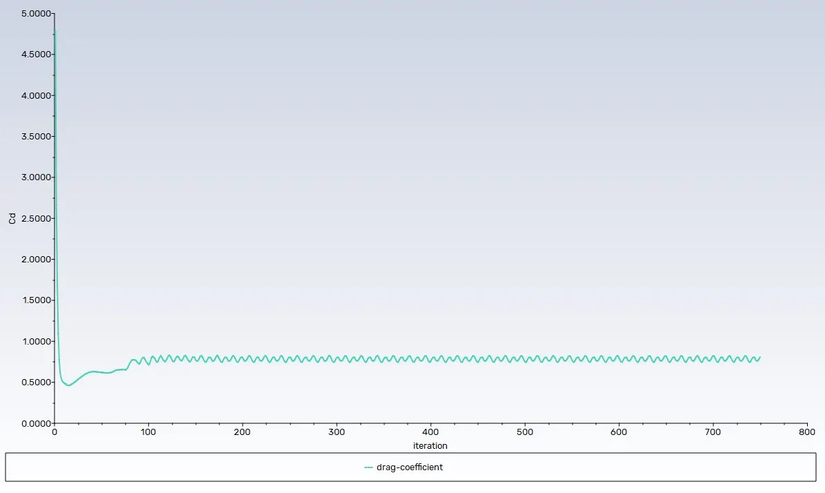
Drag co-efficient:
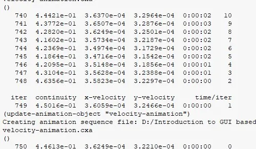
Convergence rate for X-velocity, Y-velocity and momentum:
Strouhal number:
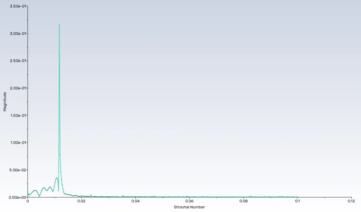
Animation:
Configuration 4: (Re = 10000)
We know that Reynold number:
Re = (ρ * V * D) / μ
Where,
ρ - density of the fluid
V - velocity of the fluid
D - diameter of the cylinder
μ - absolute viscosity of the fluid
for the data the equation will be,
10000 = (1 * V * 2) / 0.02
V = 100 m/s
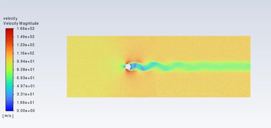
Velocity magnitude:
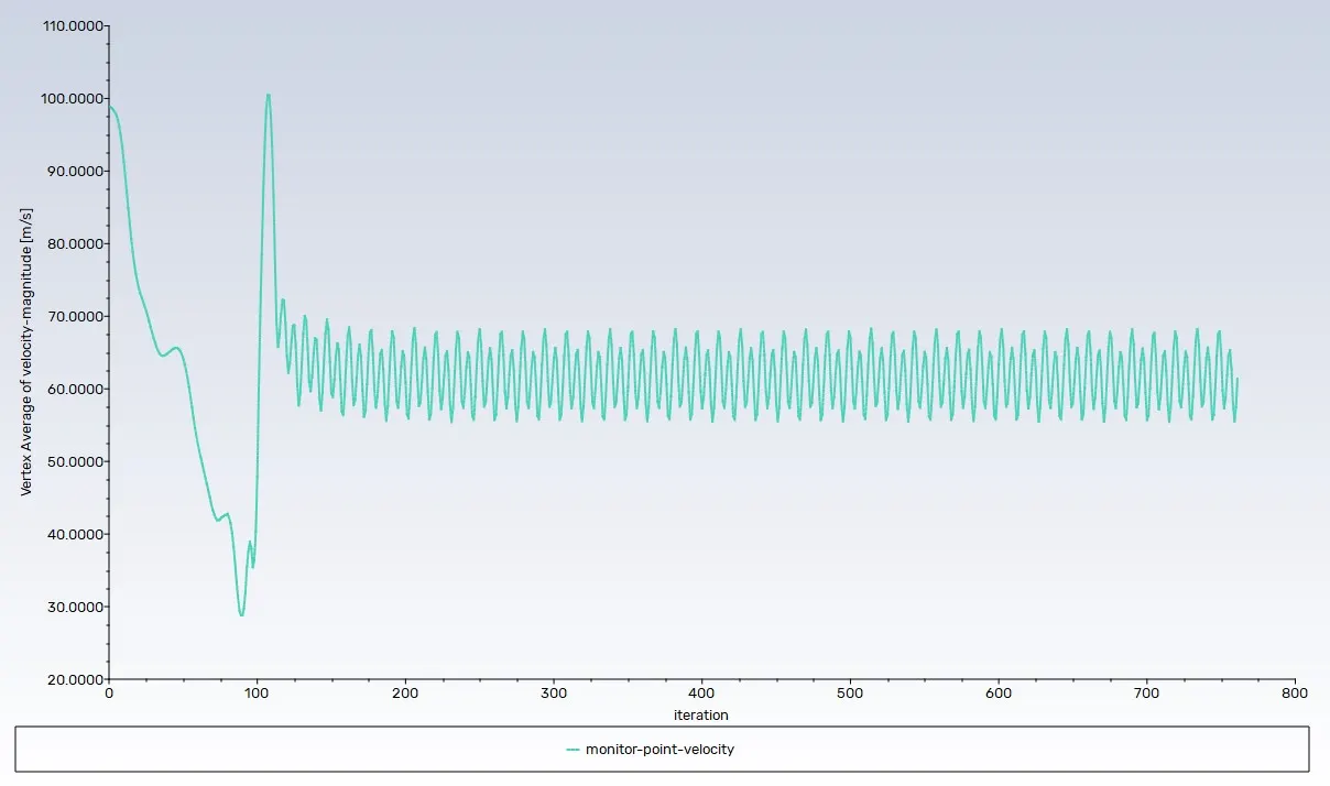
Vertex average velocity at monitor point:
Scaled residual:
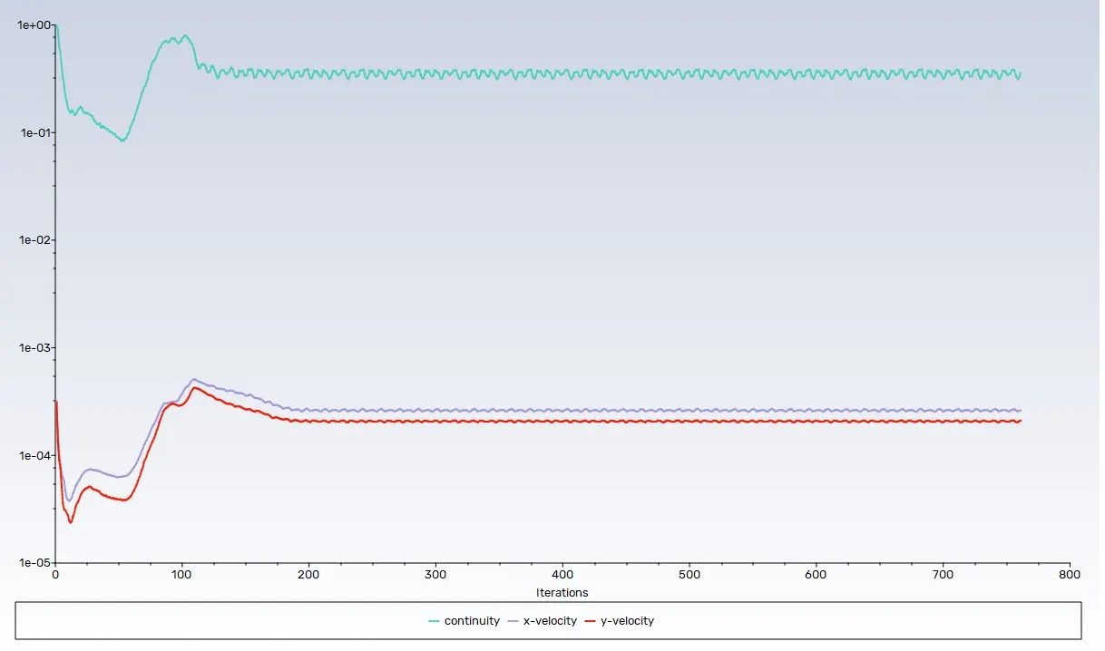
Lift co-efficient:
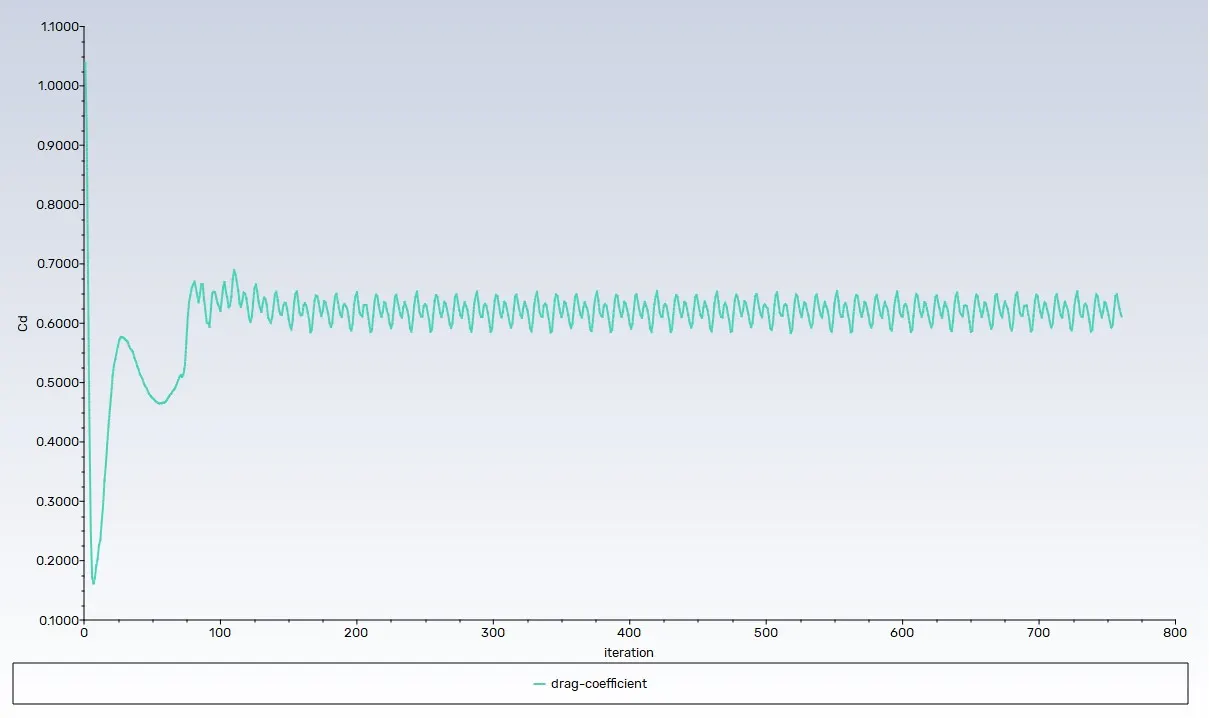
Drag co-efficient:
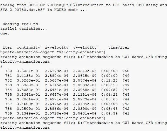
Convergence rate for X-velocity, Y-velocity and momentum:
Strouhal number:
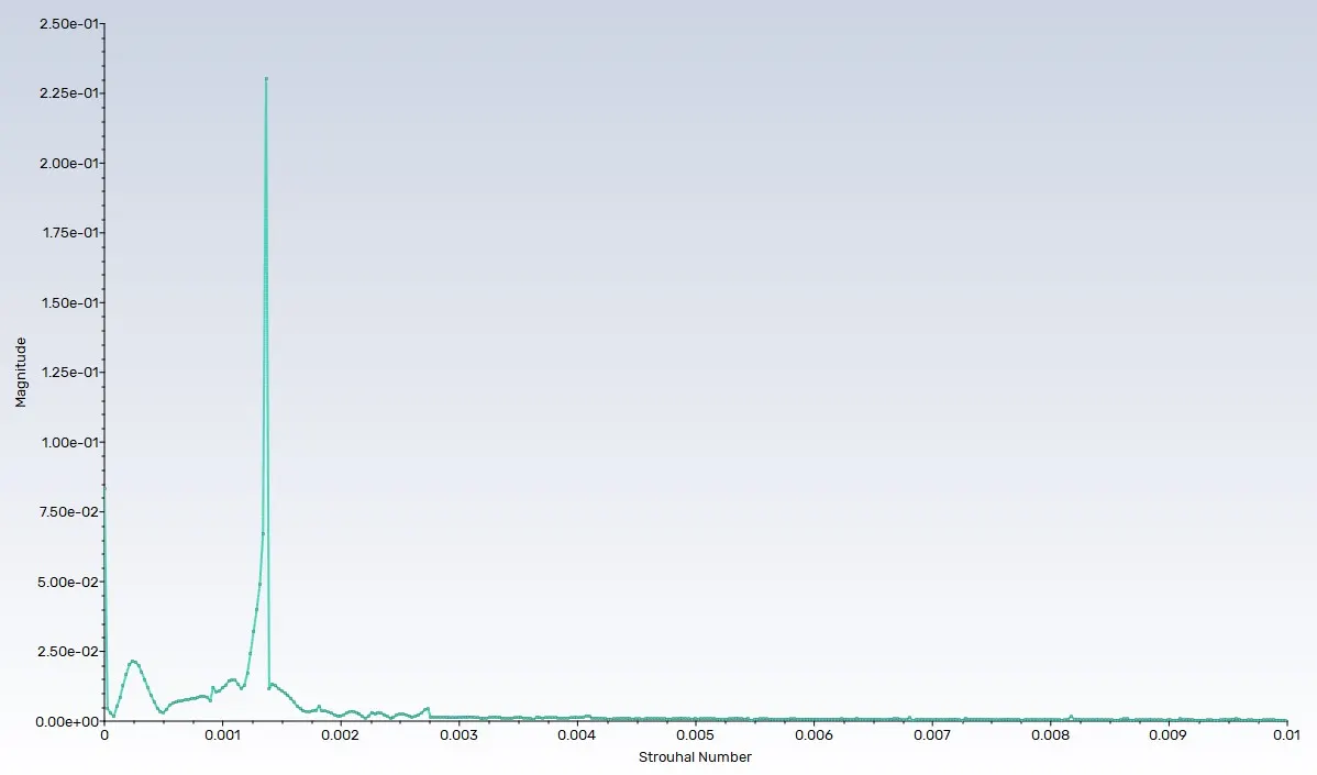
Animation:
Configuration 5: (Re = 100000)
We know that Reynold number:
Re = (ρ * V * D) / μ
Where,
ρ - density of the fluid
V - velocity of the fluid
D - diameter of the cylinder
μ - absolute viscosity of the fluid
for the data the equation will be,
100000 = (1 * V * 2) / 0.02
V = 1000 m/s
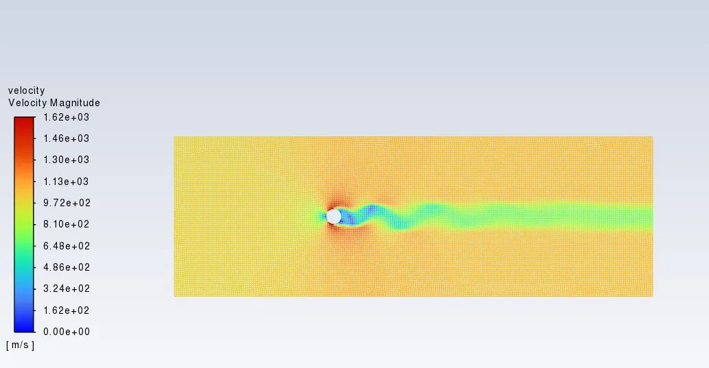
Velocity magnitude:
Vertex average velocity at monitor point:
Scaled residual:
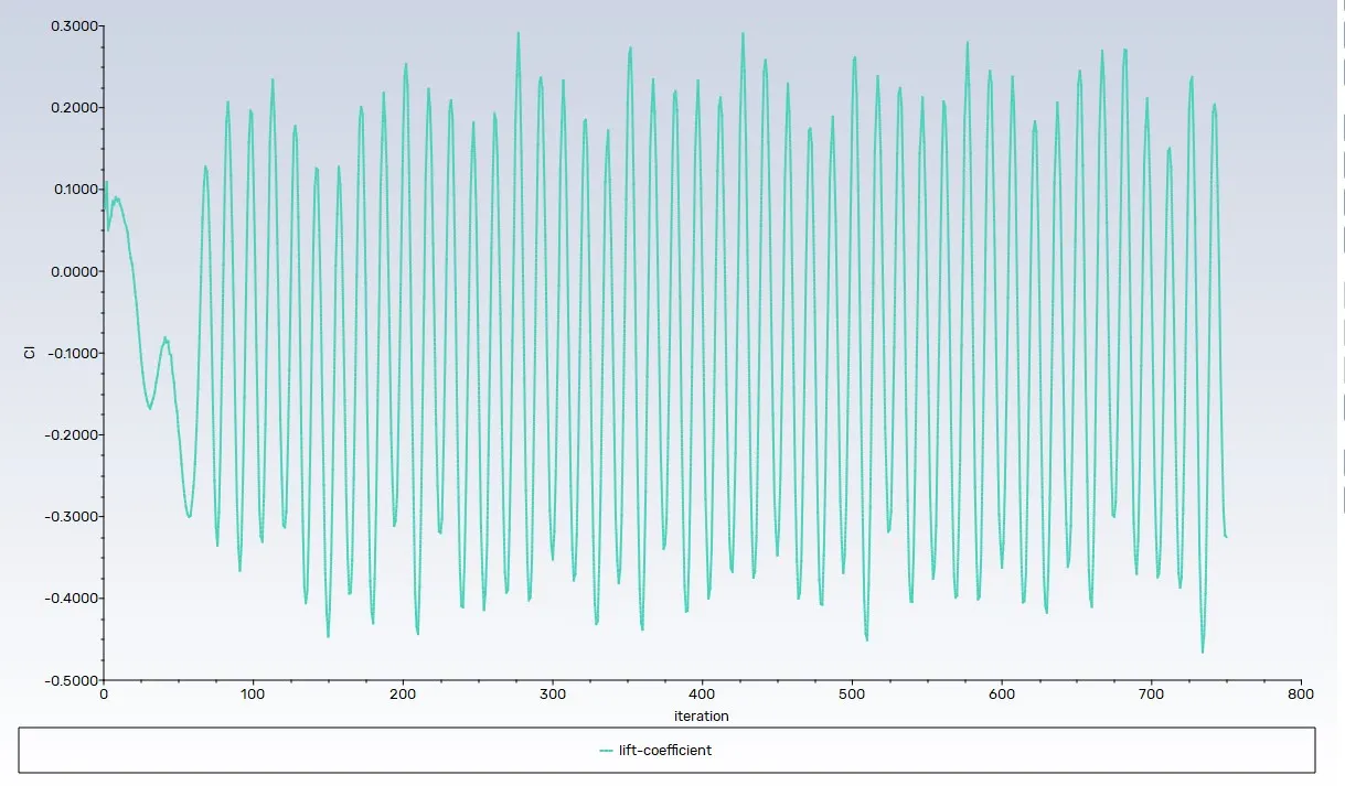
Lift co-efficient:
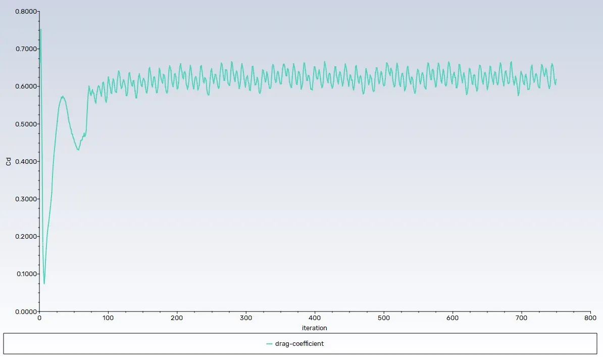
Drag co-efficient:
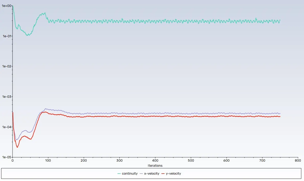
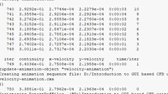
Convergence rate for X-velocity, Y-velocity and momentum:
Strouhal number:
Animation:
RESULT DISCUSSION FOR STEADY STATE Re ABOVE 100:
- at Re above ~ 47, the flow past a cylinder naturally becomes unsteady and start to exhibit vortex shedding.
- this behaviour continues and strengthens beyond Re ~ 100 entering a fully periodic regime.
- the steady state solver assumes that all flow variables (velocity, pressure, etc..) donot change with time.
- but in reality, the flow field is inherently unsteady (vortices are being shed alternately)
- the pressure and velocity fields oscillate with time, so there no single steady solution.
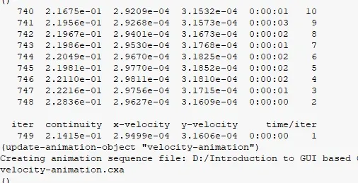
- therefore, the residuals never converged to a fixed solution, because the solver is trying to force a "nonexistent steady answer" to an "inherently unsteady problem".
FLUENT - TRANSIENT STATE (Setup) [Re - 100]:
- time derivatives are not neglected
- the solver advances the solution step by step in time, allowing the flow to evolve naturally
- at each time step, the solution may converge (inner iteration), but it captures the actual changing flow behaviour.
- hence, oscillating lift and drag and eventually reach a periodic vortex shedding pattern.
Configuration 5: (Re = 100)
We know that Reynold number:
Re = (ρ * V * D) / μ
Where,
ρ - density of the fluid
V - velocity of the fluid
D - diameter of the cylinder
μ - absolute viscosity of the fluid
for the data the equation will be,
100 = (1 * V * 2) / 0.02
V = 1 m/s
Velocity magnitude:
Vertex average velocity at monitor point:
Scaled residual:
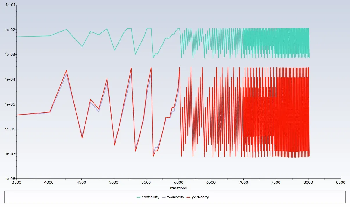
Lift co-efficient:
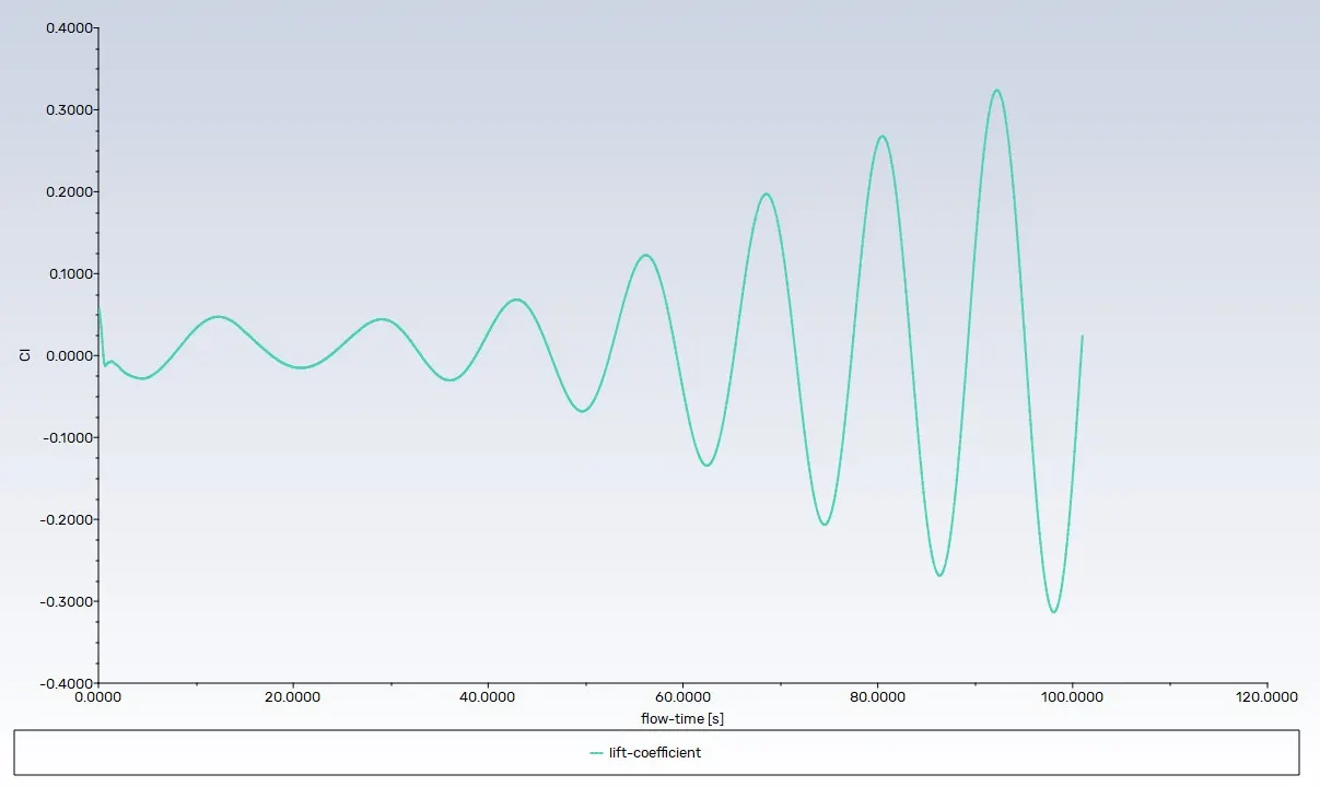
Drag co-efficient:
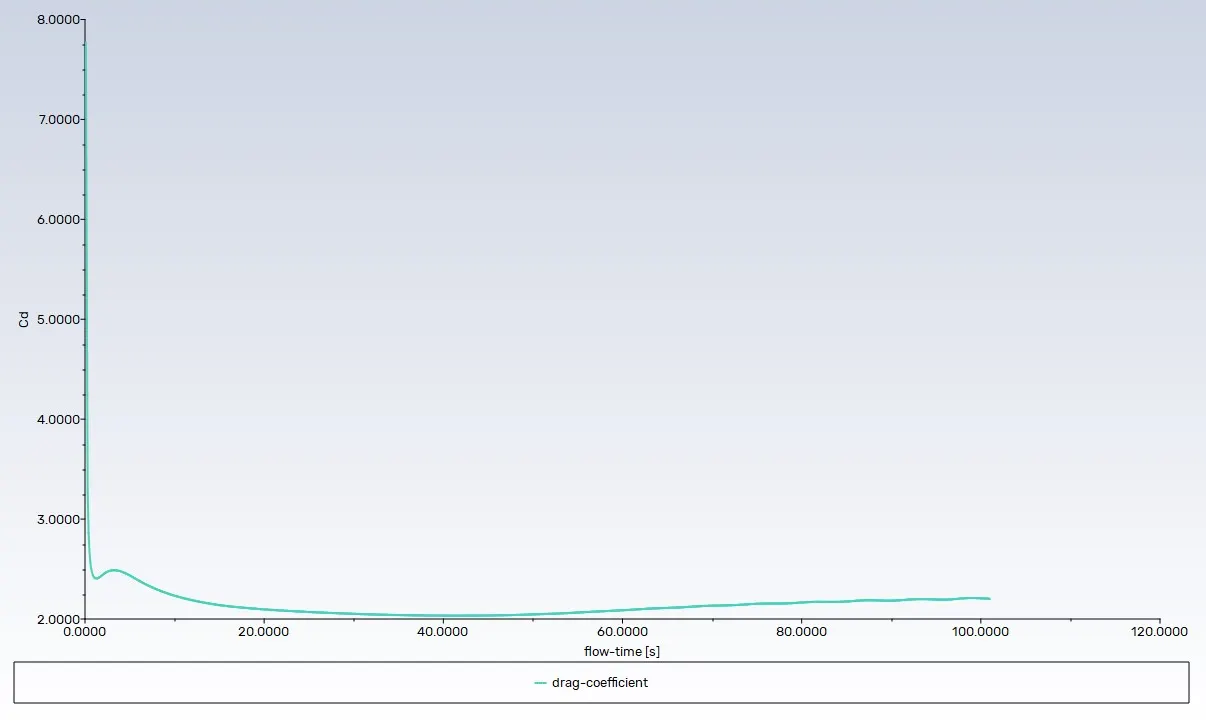
Convergence rate for X-velocity, Y-velocity and momentum:
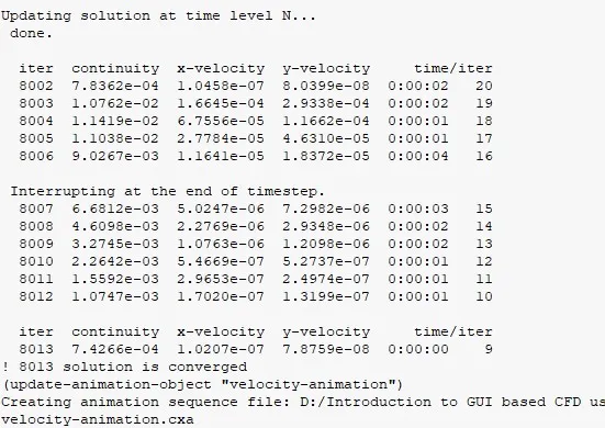
Strouhal number:
Animation:
RESULT DISCUSSION:
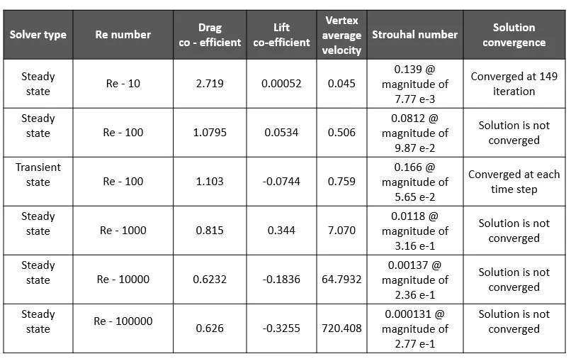
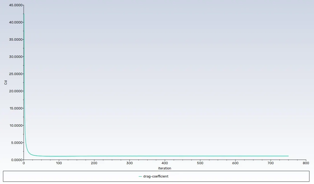
As Reynolds number increases, the drag coefficient decreases, and this behavior is due to the interplay between two types of drag:
1. Pressure drag (also called form or bluff body drag) and
2. Friction drag (due to wall shear stress).
- At low Reynolds numbers, the boundary layer is laminar and separates early from the surface, creating a large wake. This leads to high pressure drag.
- As Re increases, the boundary layer transitions to turbulent. A turbulent boundary layer has higher momentum, so it sticks to the wall longer, causing delayed separation.
- This reduces the wake size, thereby reducing pressure drag significantly — even though friction drag slightly increases due to turbulence, the overall drag decreases because pressure drag dominates for bluff bodies.
The Strouhal number must be computed using transient lift coefficient data.
- Steady-state simulations underestimate or misrepresent vortex shedding behavior and related quantities like lift, drag oscillations, and St as it is not time dependent
- as we all know there is a frequency in strouhal number formula, where f = 1/t which helps to predict the accurate frequency for strouhal number
- For Re > 47, always use transient solver to extract accurate Strouhal number (typically using FFT or zero-crossing method on CL(t).
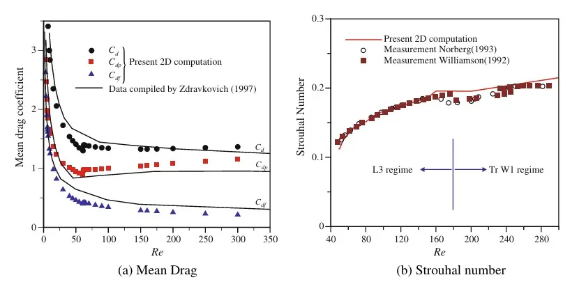
Experimental reference data:
Numerical simulation of laminar flow past a circular cylinder
Reference material:
1) https://www.sciencedirect.com/science/article/pii/S0307904X08000243
2) https://www.youtube.com/watch?v=5kcyzcDlSP8&list=PLZOZfX_TaWAE7uM59dIBr-rH73WTJCcp_&index=15
3) https://archive.org/details/FundamentalsOfAerodynamics5thEdition/page/n691/mode/2up