Week 2 - Flow over a Cylinder.

Aim: To simulate the flow of a user defined fluid over a cylinder using both steady transient solvers to calculate the Strouhal number for Reynolds number=100.

Introduction: The Karman vortex street is a phenomenon of repeating patterns of swirling vortices that is caused by vortex shedding. Vortex shedding is responsible for the unsteady separation of fluid flow around blunt objects (such as cylinders).

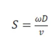
Theory: Under appropriate flow conditions around a bluff body (like the supplied cylinder model), the flow produces a regular pattern of alternating vortices. They produce a sinusoidally varying force perpendicular to the direction of flow on the body. For cylinders, the frequency ω (in Hz) of the shedding is related to the diameter D(m) and flow velocity v (ms⁻¹) via the Strouhal number ‘S’:

Applications: The designs of chimneys, bridges, and periscopes need to take this phenomenon into account.

Solving and Modelling Approach: The simulation is a 2D simulation.

For Part 1:

The schematic for Ansys fluent was opened on Ansys Workbench. For setting up the geometry, Ansys Discovery was opened. A circle was sketched with a diameter of 2m. The boundaries were further defined with the help of construction lines with the dimensions taken from the reference video. The construction lines were then deleted.

Now, the next step was to make the named selections and mesh the surface. Now for meshing this surface, three meshing methods were inserted.

All triangles method: After right clicking on ‘Mesh’ in the project tree, the insert method option was clicked. The ‘Geometry’ was selected to be the entire surface (both the body selection and face selection tool can be used as it is only a 2D body). Then the setting in the ‘Method’ option was changed from ‘Quadrilateral Dominant’ to ‘Triangles’.

Sizing method: To capture the geometry along the cylinder’s perimeter better, this option was used.

The ‘Geometry’ to be applied on was selected to be the circular edge using the edge selection tool.

The setting on ‘Type’ was set to ‘Number of Divisions’, and this was set to 36 divisions (I division for every 10 degrees of rotation about the circular perimeter’s centre.

Inflation Layer: This method is used to create a ‘Boundary Fitted’ mesh. The ‘Geometry’ to be applied on was again selected to be the entire 2D face and the ‘Boundary’ was selected to be the edge of the circle. The setting for ‘Inflation Option’ was set to be ‘First layer Thickness’ and the ‘First Layer Height’ was defined to be 5mm. The ‘maximum layers’ was set to 6, the growth rate was not changed from the default setting of 1.2.

After setting the element size to 0.5mm, the mesh was generated.

On moving on to the Set-Up option in the schematic, the launcher opens. ‘Double precision’ was checked and the number of processors was increased to 5 (processing option was set to parallel).

In the solver settings, we select ‘Pressure Based’ for the ‘Type’. The ‘Velocity Formulation is set to ‘Absolute’. And the ‘Time’ is set to ‘Steady’.

Since, we are working with low Reynolds number regimes, the viscous model is set to ‘Laminar’.

In the ‘Materials’ group, we select the ‘Create/Edit’ option. From, the fluent database, we copy the properties for air and name this new material “user-material”. The density is defined to be 1kg/m^3.

The viscosity is set to be 0.02.

In the ‘Cell Zones’ option, we change the ‘Material Name’ from ‘air’ to ‘user-defined’.

The ‘Boundary Conditions’ were set up as follows;

Wall: It was made sure that the ‘No Slip’ condition was checked.

Symmetry: The ‘Type’ was set to ‘Symmetry’ (automatically done by fluent due to the named selection).

Outlet: the ‘Gauge Pressure’ was set to 0.

Inlet: The ‘Velocity Magnitude’ was set to be 1m/s.

In the ‘Results’ tab, from the ‘Create’ option, a point was created to be monitor point.

The coordinates for this point were set to be “(8,0)” with the origin being the centre of the circle.

A new ‘Surface Report’ was created of the type ‘Vertex Average’. With the field variable set to be ‘Velocity’ for the monitor point created.

In the ‘Residuals’ options in the ‘Reports’ section in the ‘Solution’ tab, all the boxes for ‘Check Convergence’ were unchecked.

The solution was then initiated (‘Hybrid’ type). Using these initial values, contours for pressure and velocity for the entire surface were created along with an animation to study the vortewx shedding more closely. The number of iterations were set to 1400 in hopes of getting a converged solutions.

Density of defined material: 1 kg/m^3

Velocity of flow: 1m/s

Diameter of cylinder: 2m

Viscosity: 0.02kg/ (m*s)

Therefore, the Reynold’s number for the flow of this fluid around the cylinder comes out to be 100.

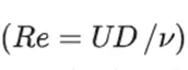
Where ‘U’ is the free stream velocity, ‘ν’ is the kinematic viscosity and ‘D’ is the diameter of the cylinder.

Results:

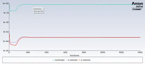
The solution was not converging even after 1400 iterations. The plots for both residuals and vertex average of velocity were oscillating. The residuals were also not small in magnitude.

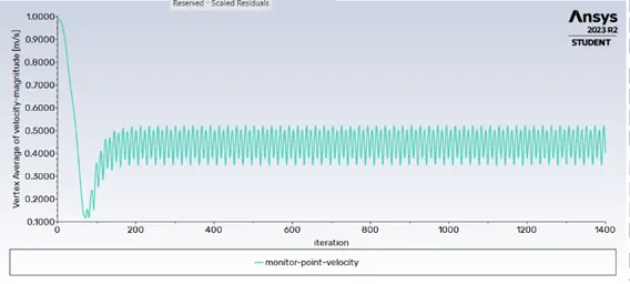
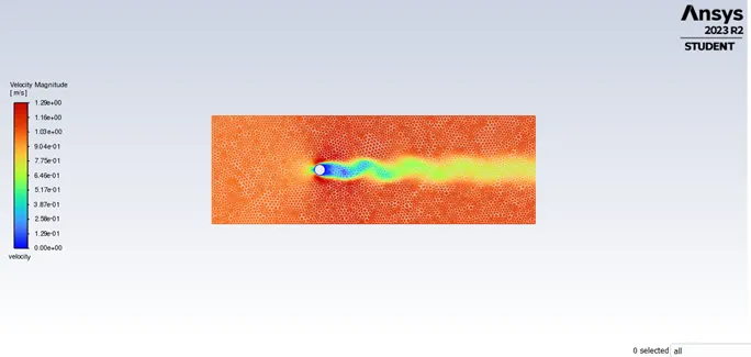
The solver was now set up for a Transient simulation. The time step was size was set to 0.1 and the calculation were carried out again;

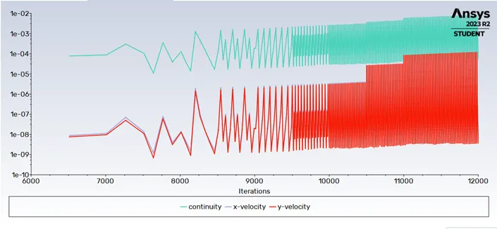
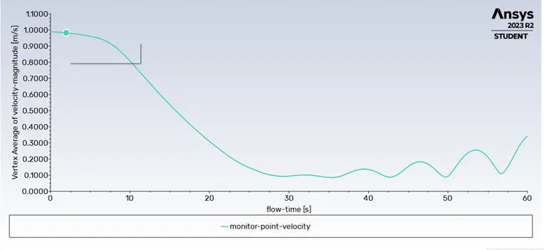
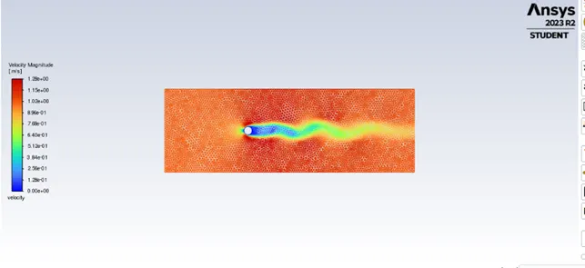
From the plot for vertex average of velocity, the frequency can be calculated to be 0.182/s.

(0.182=5/27.5; observing the peaks from 32.5 seconds to 60 seconds).

Using this in the formula for Strouhal number 0.182*2/1=0.364

To calculate the coefficient of drag:(Part-2)

For Re=10.

The viscosity of the “user-material” was set to 0.05Kg/(m*s).

The inlet velocity was set to 2.5m/s so that the calculated Reynold’s number would be 10.

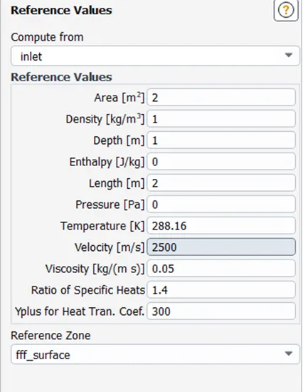
The reference values were set accordingly:

(The velocities were varied case by case to get the desired value of Reynold's number).

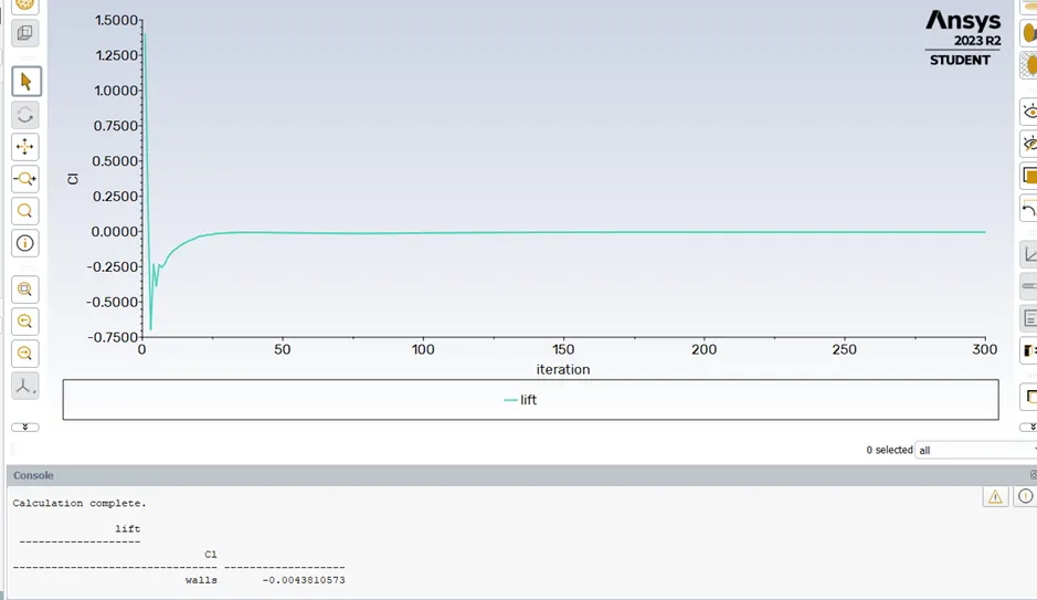
The computed value of Cl=-0.0043810573.

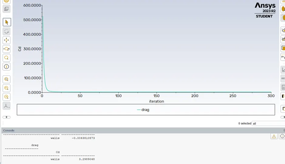
The value if Cd= 3.2989048.

For Re=100;

The inlet velocity was upped to 2.5m/s so that the calculated Reynold’s number would be=100.

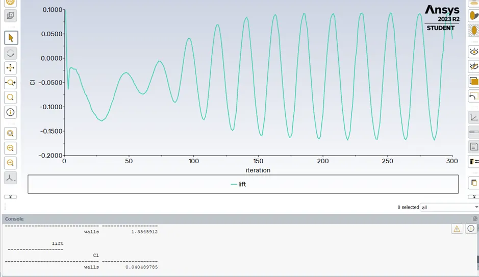
Cl= 0.040489785.

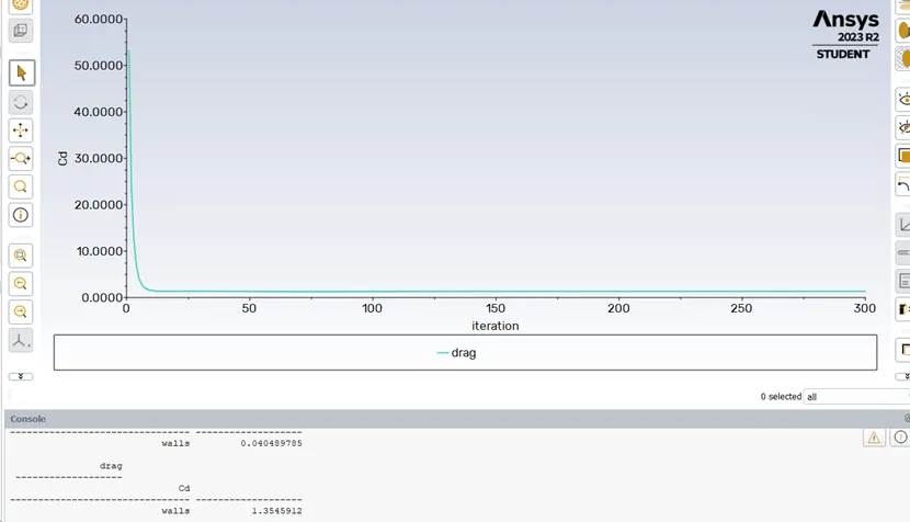
The computed value of Cd= 1.3545912.

For Re=1000;

The inlet velocity was upped to 25m/s so that the calculated Reynold’s number would be=1000.

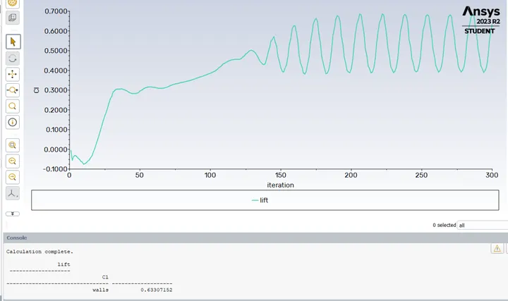
Cl= 0.63307152.

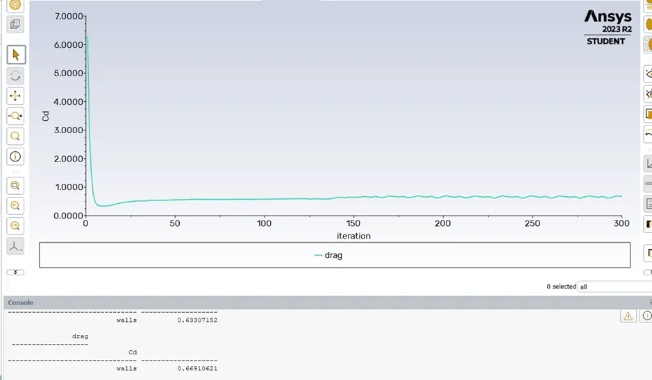
Cd= 0.66910621.

For Re=10000;

The inlet velocity was upped to 250m/s so that the calculated Reynold's number would be 10000.

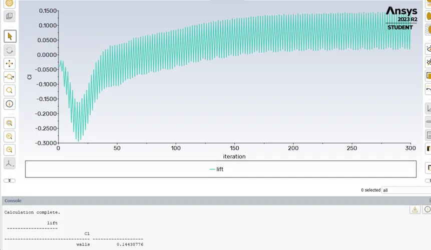
Cl= 0.14438776.

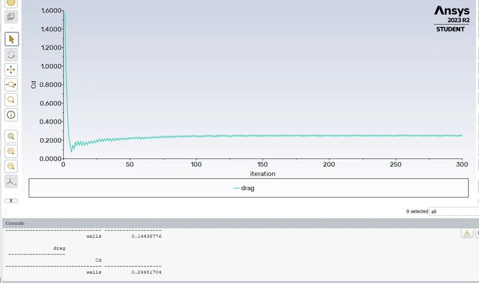
Cd= 0.24481704.

For Re=100000;

The inlet velocity was changed to 2500m/s so that the calculated value of Rwynold’s number would be 100000.

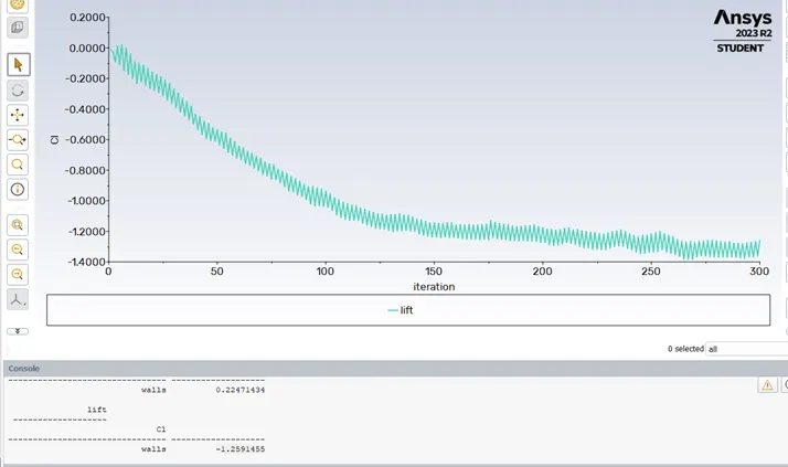
Cl= -1.2591455.

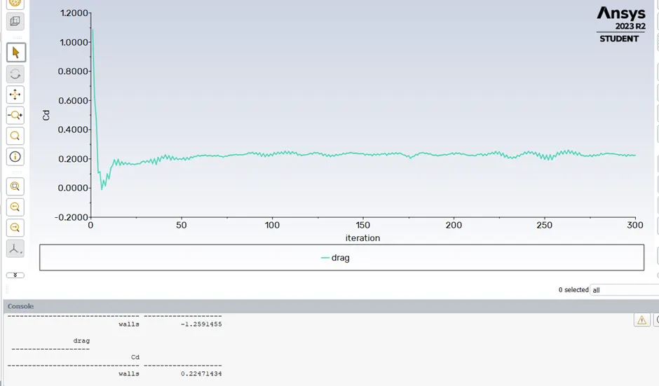
Cd= 0.22471434.

Observations and Results:

For Re=10, the Coefficient of Drag for the cylinder was around 3.3. It kept decreasing as the Reynold’s number was increased case by case.