Week 2 - Flow over a Cylinder.
OBJECTIVES: -
Simulate the flow over a cylinder and explain the phenomenon of Karman vortex street.
PART-I
Simulate the flow with the steady and unsteady case and calculate the Strouhal Number for Re= 100.
PART-II
Calculate the coefficient of drag and lift over a cylinder by setting the Reynolds number to 10,100,1000,10000 & 100000. (Run with steady solver)
Discuss the effect of Reynolds number on the coefficient of drag. [ Results should be validated with any standard literature and error should be within 5 %]
Expected results:-
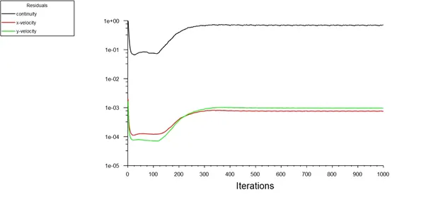
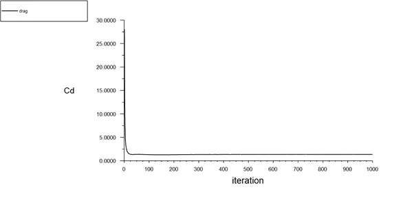
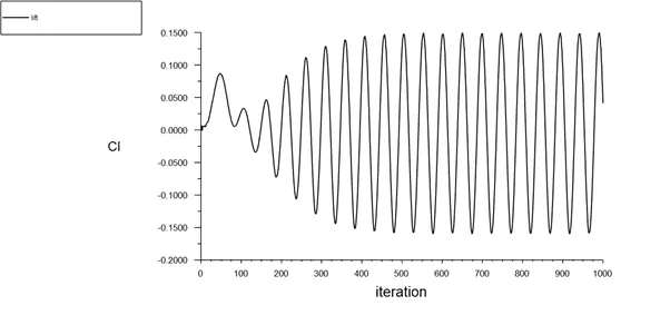
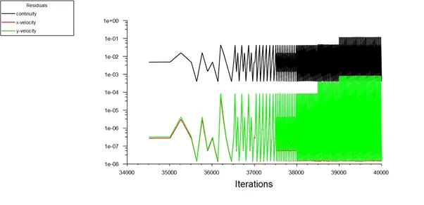
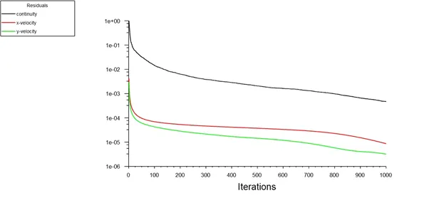
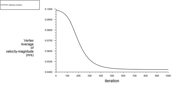
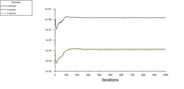
In both approaches, show that the flow has converged. That is, what quantities or plots need to be looked at to determine that the flow has converged?
Plots of the coefficient of drag and lift.
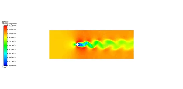
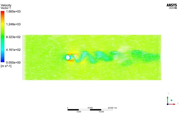
Plots to show vortex shedding behind the cylinder.
Mention the referred material at the end of the challenge submission page.
INTRODUCTION
Flow over cylinder
Separated flows is one of the most complex problems studied in fluid dynamics and has been the most researched area in past years. Fluid flow past a circular cylinder is a model problem of fundamental interest, as it impacts a number of practical engineering applications like heat exchangers, condensers, economizers, nuclear reactor fuel rods etc.
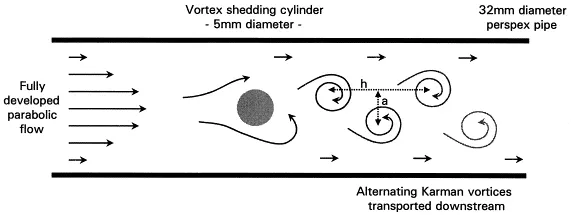
The flow past a circular cylinder is associated with various instabilities. Vortices are formed and shed behind the cylinder wall and gives rise to fluctuating drag and lift forces. It is well known that the vortex wake information of a circular cylinder can be studied as the function of the Reynolds number. The first definition of flow regimes based on measurement of velocity fluctuations spectra and frequency was given by Roshko (1954). He found a periodic laminar vortex shedding regime for Re = 40 -150; a transition regime in the range Re = 150 -300 and irregular regime for Re = greater than 300, where velocity fluctuations showed distinct irregularities. The sharpness of cylinder corners in the experiments and the numerical analysis considerably influences the shedding frequency. Understanding the wake behaviour and the associated dynamics of flow past cylinder helps in the better design of the concerned or desired objectives, where the engineering parameters need to be designed with reasonable precision.
Coefficient of drag
In fluid dynamics, the drag coefficient is a dimensionless quantity that is used to quantify the drag or resistance of an object in a fluid environment, such as air or water. It is used in the drag equation in which a lower drag coefficient indicates the object will have less aerodynamic or hydrodynamic drag. The drag coefficient is always associated with a particular surface area.
The drag coefficient is represented as: -
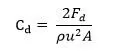
Where Fd is the drag force
ρ is the mass density of fluid
U is the flow speed
A is the reference area
The drag coefficient of any object comprises the effects of the two basic contributors to fluid dynamic drag: skin friction and form drag.
Coefficient of lift
The lift coefficient is a dimensional coefficient that relates the lift generated by a lifting body to the fluid density around the body, the fluid velocity and an associated reference area. A lifting body is a foil or a complete foil bearing body such as a fixed – wing aircraft. Coefficient of lift is a function of the angle of the body to the flow, its Reynolds number and it’s Mach number.
Mathematically it is represented as: -
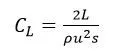
Where L is the lift force
S is the relevant surface area
ρ is the fluid density
u is the flow speed
Strouhal number
Strouhal number is a dimensionless number which represents the ratio of inertial forces due to the local acceleration of the flow to the inertial forces due to convective acceleration. In flows characterized by a periodic motion, the strouhal number is associated with the oscillations of the flow due to the inertial forces relative to the changes in velocity due to the convective acceleration of the flow field.
The mathematical expression for strouhal number is

Where f is the frequency of the oscillations
L is the characteristic length
U is the flow velocity.
GEOMETRY
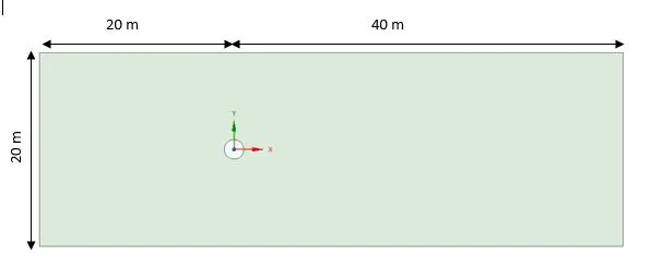
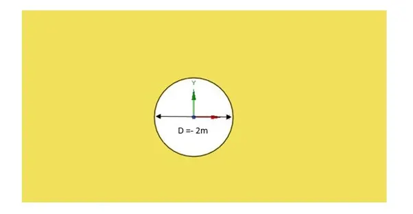
The schematic of the side view of the model has been shown in the figure below. The diameter of cylinder is 2m. The upstream length has been kept 20m and downstream is 40m to ensure that the vortex shedding is captured properly. In the present simulation 2D analysis has been carried out as the two dimensional and three dimensional CFD analysis yield very close results. Furthermore, 2D analysis can be adopted instead of 3D analysis to save computer memory and computational time.
MESHING
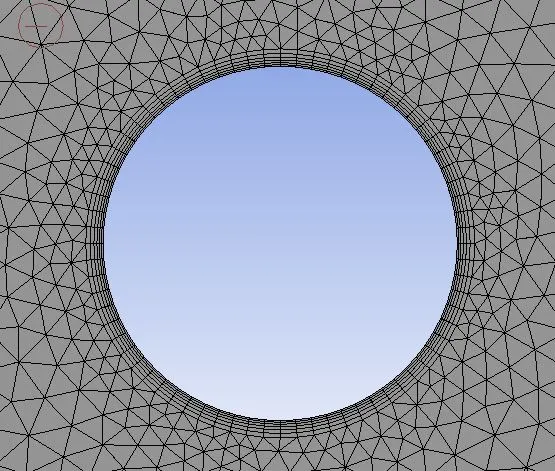
The triangle method has been used to mesh the computational domain. Details of mesh has been provided below.
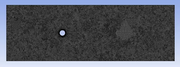
Mesh size = 0.25 mm
Number of inflation layers = 6
Growth rate = 1.2
CASE SETUP
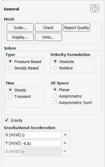
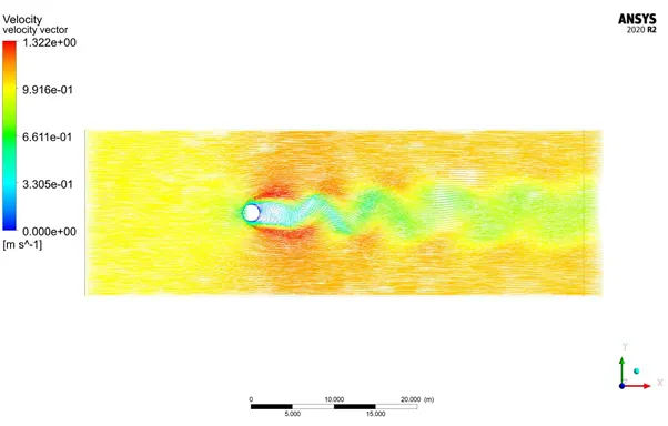
The simulation has been performed for both steady and unsteady cases. From the literature we know that laminar vortex shedding is observed between Re = 40 -150, analysis has been carried out at Re = 100 for both steady and unsteady cases. To study the effect of Reynolds number on the instabilities formed in the wake region of cylinder wall, the simulation has been performed for steady case varying the Re from 10 to 100000. The snippets provided below shows the steps to setup the case in fluent.
Solver – pressure based solver
Time – steady
Gravity – 9.81 in negative y direction
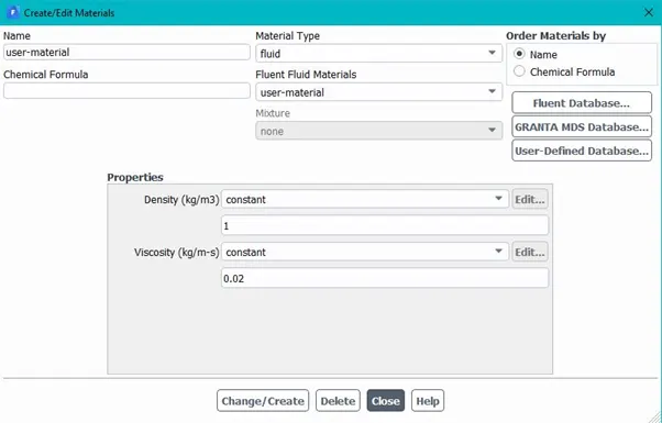
To create user material create material option is used.
Density = 1kg /mm3
Viscosity = 0.02
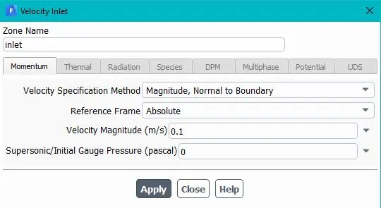
Inlet velocity has been varied according to Reynolds number.
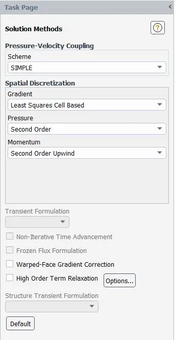
Pressure velocity coupling = SIMPLE algorithm
Pressure discretization = second order
Momentum discretization = second order upwind
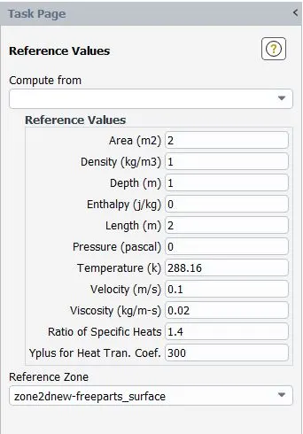
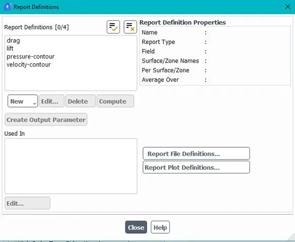
Reference values has to be input correctly to get the accurate values of drag and lift coefficient
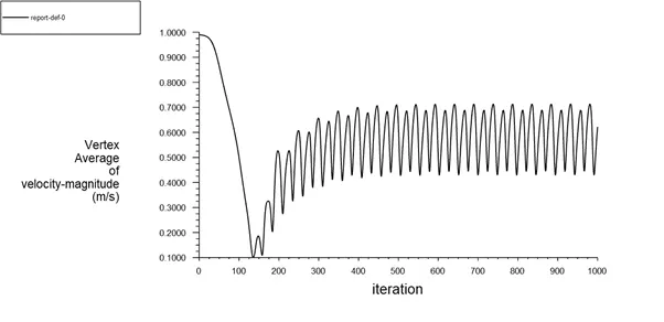
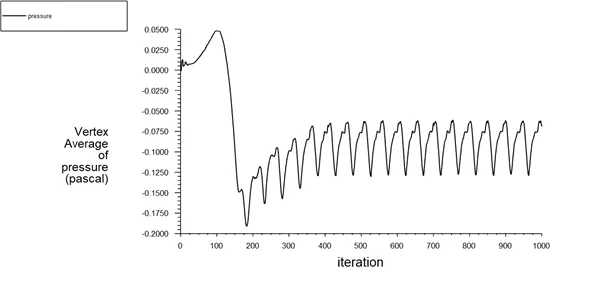
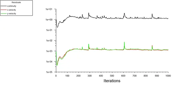
Various graphs has been plot to monitor the convergence.
RESULT AND DISCUSSIONS
PART 1
CASE 1: -
TIME: - STEADY STATE
RE = 100
V = 1 m/s
Residual plot
 Velocity plot
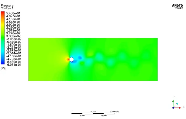
Pressure plot
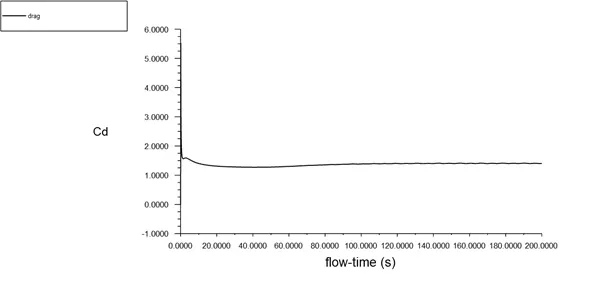
Coefficient of drag plot
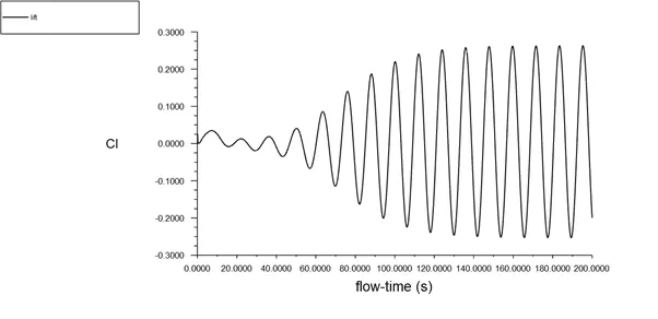
Coefficient of lift plot
Velocity contour
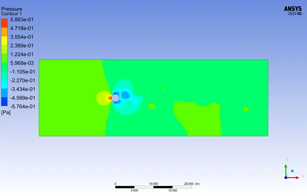
Pressure contour
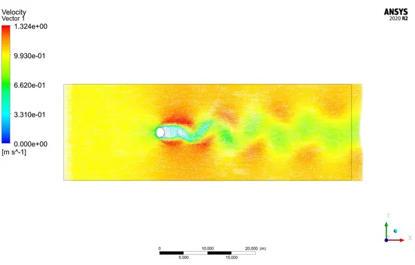
Velocity vector
Case 2: -
Time – unsteady
RE = 100
V = 1 m/s
Residual plot
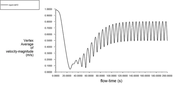
Velocity plot
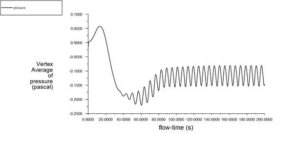
Pressure plot
Coefficient of drag
Coefficient of lift
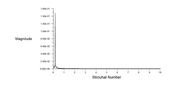
Strouhal plot
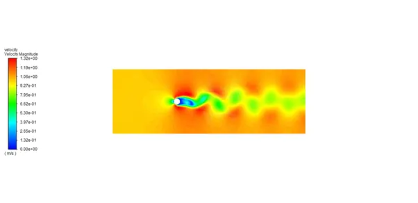
Velocity contour
Pressure contour
Velocity vector
Calculation of strouhal number
f = number of cycle /time
f = 5/50
= 0.1
S = (0.1 × 2)/1 = 0.2
Part 2
CASE 1: -
TIME: - STEADY STATE
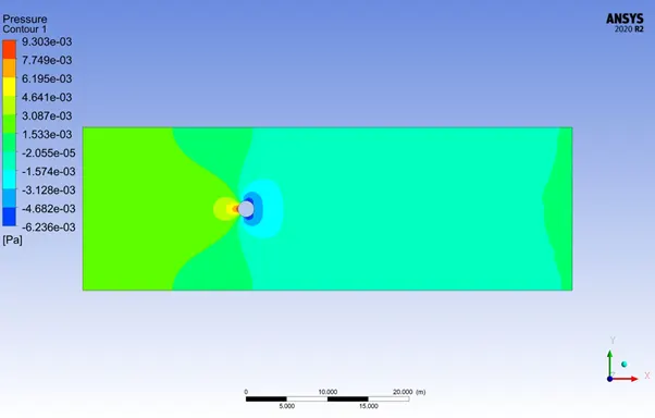
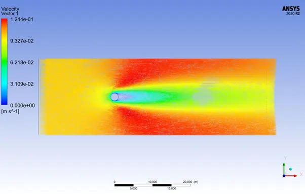
RE = 10
V = 0.1 m/s
Residual plot
Velocity plot
Pressure plot
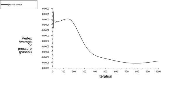
Coefficient of drag
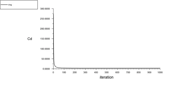
Coefficient of lift
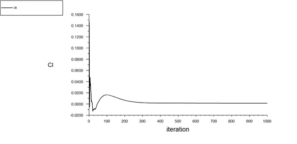
Velocity contour
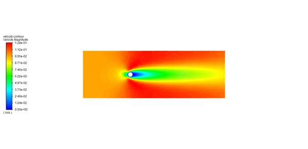
Pressure contour
Velocity vector
CASE 2: -
TIME: - STEADY STATE
RE = 100
V = 1 m/s
Residual plot
Velocity plot
Pressure plot
Coefficient of drag
Coefficient of lift
Velocity contour
Pressure contour
Velocity vector
CASE 3: -
TIME: - STEADY STATE
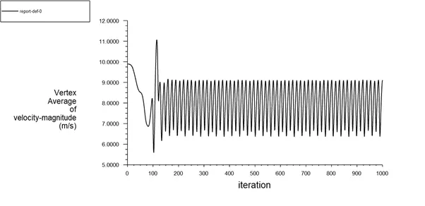
RE = 1000
V = 10 m/s
Residual plot
Velocity plot
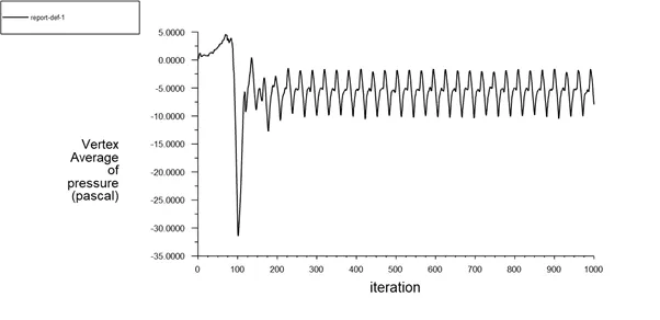
Pressure plot
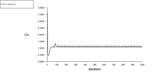
Coefficient of drag
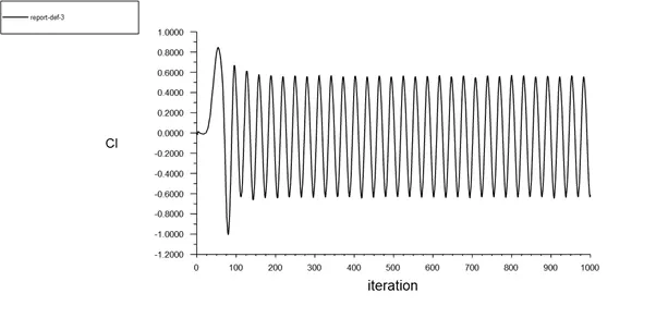
Coefficient of lift
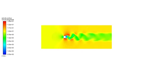
Velocity contour
Pressure contour
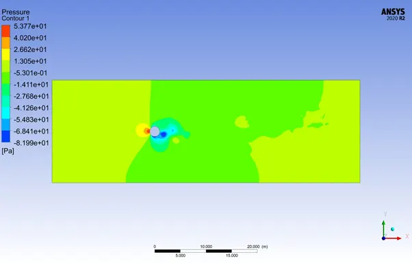
Velocity vector
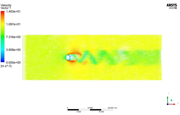
CASE 4: -
TIME: - STEADY STATE
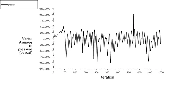
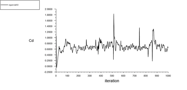
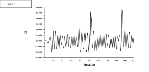
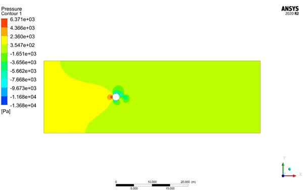
RE = 10000
V = 100 m/s
Residual plot
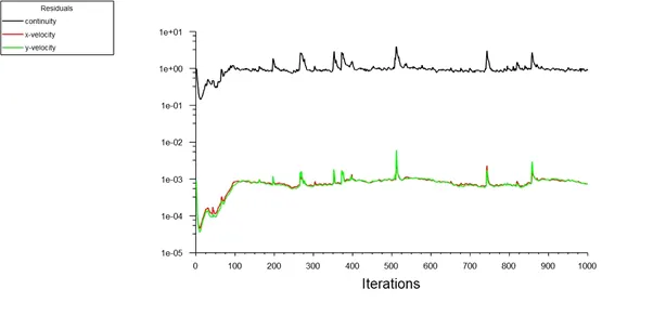
Velocity plot
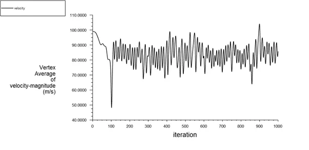
Pressure plot
Coefficient of drag
Coefficient of lift
Velocity contour
Pressure contour
Velocity vector
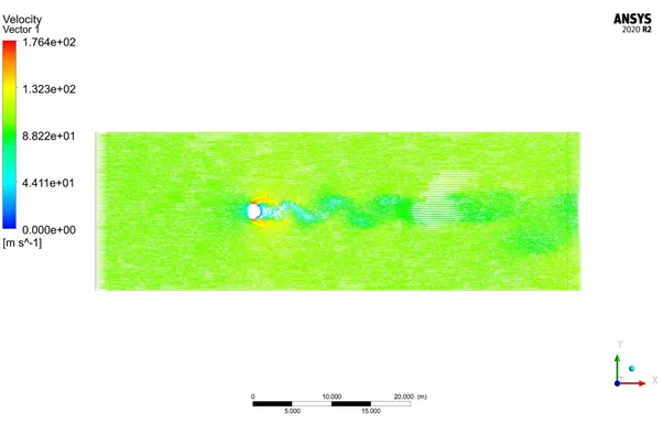
CASE 5: -
TIME: - STEADY STATE
RE = 100000
V = 1000 m/s
Residual plot
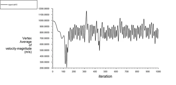
Velocity plot
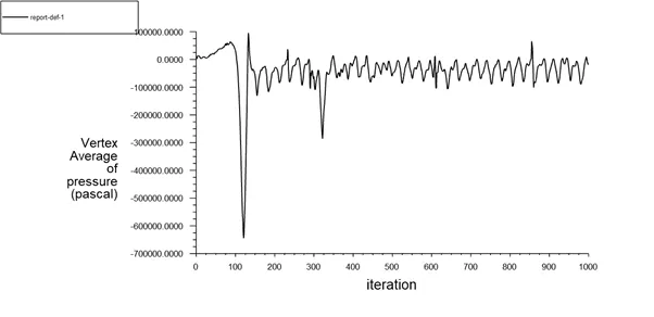
Pressure plot
Coefficient of drag
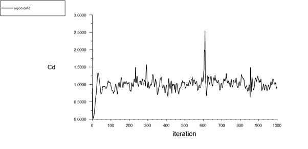
Coefficient of lift
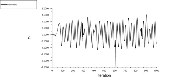
Velocity contour
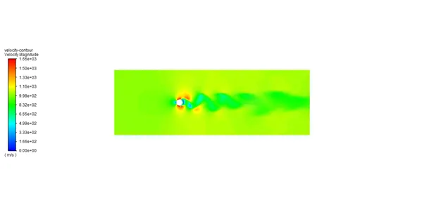
Pressure contour
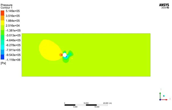
Velocity vector
The table below shows the change in drag coefficient and lift coefficient with variation in Reynolds number
|
RE (STEADY STATE) |
COEFFICIENT OF DRAG (Cd ) |
COEFFICIENCT OF LIFT (Cl) |
|
10 |
3.344208
|
0.003564
|
|
100 |
1.405399
|
0.002794
|
|
1000 |
0.681085 |
0.027401
|
|
10000 |
1.098622
|
-0.01513
|
|
100000 |
1.005727
|
0.071499
|
Validation with respect to the reference paper.
| Re | Theoritical Cd | numerical Cd | error |
| 10 | 3.5 | 3.34 | 4.5% |
| 100 | 1.335 | 1.4 | 4.8% |
CONCLUSIONS
1) No vortex shedding is observed at Re =10.
2) vortex shedding is observed at higher value of Re =100. The strouhal number calculated for the unsteady case is found to be around 0.2.
3) with the increment in reynolds number drag coefficient decreases significantly attains a minimum value and againg shows slight increment.
4) validation with respect to literature shows error less than 5% which signifies the veracity of present simulation.
5) using finer mesh may help in getting more accurate results.
REFERENCES
B.N.Rajani A.Kandasamy SekharMajumdar, " Numerical simulation of laminar flow past a circular cylinder" Applied mathematical modelling 33 (2009) 1228-1247