Week 2 - Flow over a Cylinder.

AIM:

In this week's challenge, we have to Simulate the flow over a cylinder and we also need to explain the phenomenon of Karman vortex street.  

PART-I

1. Simulate the flow with the steady and unsteady case and calculate the Strouhal Number for Re= 100. 

PART-II

1. Calculate the coefficient of drag and lift over a cylinder by setting the Reynolds number to 10,100,1000,10000 & 100000. (Run with steady solver)
2. Discuss the effect of the Reynolds number on the coefficient of drag. [ Results should be validated with any standard literature and error should be within 5 %]

Expected results:-

1. In both approaches, show that the flow has converged. That is, what quantities or plots need to be looked at to determine that the flow has converged?
2. Plots of the coefficient of drag and lift. 
3. Plots to show vortex shedding behind the cylinder. 
4. Mention the referred material (Reference Paper or Fluid Mechanics Textbook) at the end of the challenge submission page. 

INTRODUCTION:-

• Flow over a cylinder:

The flow over a cylinder is an external flow analysis. so, the flow passes through a two-dimensional cylinder to the outlet. In this flow-over cylinder, we have several aspects of the domain constituted as boundaries. so, it contains an inlet, outlet, wall, and cylinder. 

- Inlet: this is where the flow comes from and passes into the domain. In this case, we can provide inlet velocity.

- Outlet: this is where the flow goes out of the domain. In this case, we can provide outlet pressure.

- Wall: this is the boundary of the domain, through which flow cannot pass. this represents a physical wall, through which the information can't be passed through.

- Cylinder: A cylinder will act like a wall, as the flow can't pass through.

THEORY:-

• Reynolds number:

The Reynolds (Re) number is a dimensionless number, defined as a ratio of inertial force to viscous force. so, the idea is to understand the impact of flow trying to move in a domain and its inherent friction force (velocity) trying to stop the flow from in the domain. 

Re = (ρ.V.D)/μ

Here, 

ρ(rho) is the density of the fluid.

V is the velocity of the fluid.

D is the diameter of the cylinder.

μ(mu) is the dynamic viscosity. 

1.  Laminar (Re < 2300>
2. Turbulant (Re > 4000 - internal flow, Re > 5x105 - External flow)

and the wake region is turbulent. 

• Strouhal number:

The Strouhal number indicates the frequency of the flow to the velocity of the flow, if the frequency of the vertex shading becomes equal to the resonant frequency of the body instability will start to occur in the body where the body will start to fluctuate as well.

S.F = (ω.d)/u

Here,

ω is the Frequency of the vortex shedding

d is characteristics of length

u is flow velocity.

And to find the frequency value of F = No.of.cycle/Time interval

Here,

No.of.cycle = 6.

Time interval (sec) = 30.

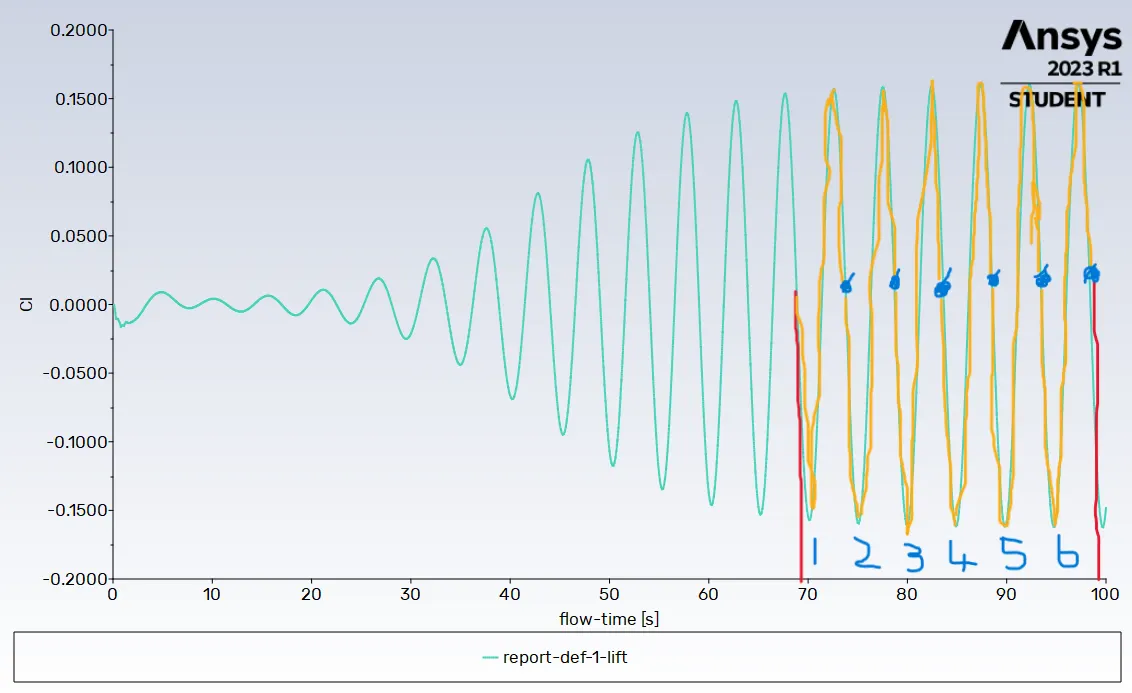
• To find the Strouhal number for Re = 100, Velocity = 2.5. And this is an unsteady state. so, The no.of cycles taken for 30 sec. and this 30 sec is the approximate time. so, the no.of.cycles for Co-drag is 6 cycles.
• so, F=6/30 is equal to 0.2 and now substitute this F value into the Strouhal number formula in ω place.
• (i.e), 0.2 x 2 / 2.5 = 0.16 
• so the Strouhal number for Re = 100 is 0.16.

 

• von Karman vortex street:

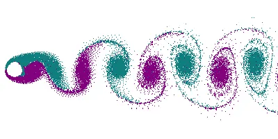
The vortex shading is a phenomenon occurring when the flow encounters a body. in the vortices are shed alternatively downstream of the flow behind the body. these low-pressure zones give rise to fluctuations in the body as the force acts at the right angle to the direction of the flow. the shedding is categorized into 4 groups based on the flow they are,

1. Below sub-critical(Re<300>
2. Sub-Critical(300
3. Transition(1.5e5
4. Supercritical(Re>3.5e6)

• What is the boundary layer?

The boundary layer is the concept of flow physics happening near the walls. when the flow passes over a boundary (Wall) the flow will try to stick to the walls. (this phenomenon is known as no-slip conditions). so, this leads to flow-changing properties as one keeps moving away from the wall. The boundary layer is very important to capture properly in CFD, as there is a sharp change in properties from near the wall to away from the wall.

• What is y+value?

The concept of y+ is tried in the boundary layer theory. When the fluid flows over a wall, it tries to stick to the wall (this phenomenon is known as no-slip conditions). during this condition, the subsequent layer of the fluid, above the one gets stuck to the wall. so this will have hindrance in their motion. This causes sharp changes in the properties of the fluid as one travels away from the wall. 

• What is the co-efficient of Drag?

the drag is a measure of resisting force to the movement of the body. Several factors may be affecting the drag force being applied to a body. Namely, the type of material of the body, shape of the body, velocity of the flow, density of the flow, viscosity of the fluid, and others.

F_D=(1/2).ρ.V².A.Cd

Here,

F_D = drag force.

ρ = Density

V = Velocity

A = cross-section area

C_D = coefficient of drag.

• What is the co-efficient of Lift?

The coefficient of lift is generated on an object concerning the density and velocity of the fluid flow.

PROCEDURE:-

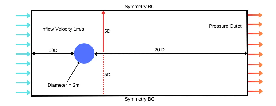
• So, we will have an inlet velocity of 1m/s, and at the outlet, we have a pressure boundary condition. and at the top and bottom, we are called the symmetry boundary conditions.

THE CFD STAGES:-

1. Pre-processing(geomentry, meshing)
2. Solving(setup, solving)
3. Post-processing(result)

MODELING APPROACH:

1. Pre-processing(geomentry, meshing)

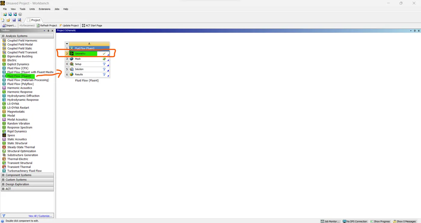
• so, open the ansys fluent software, then drag and drop the fluid flow (fluent), and double click the "geomentry" to open the geomentry GUI.

 

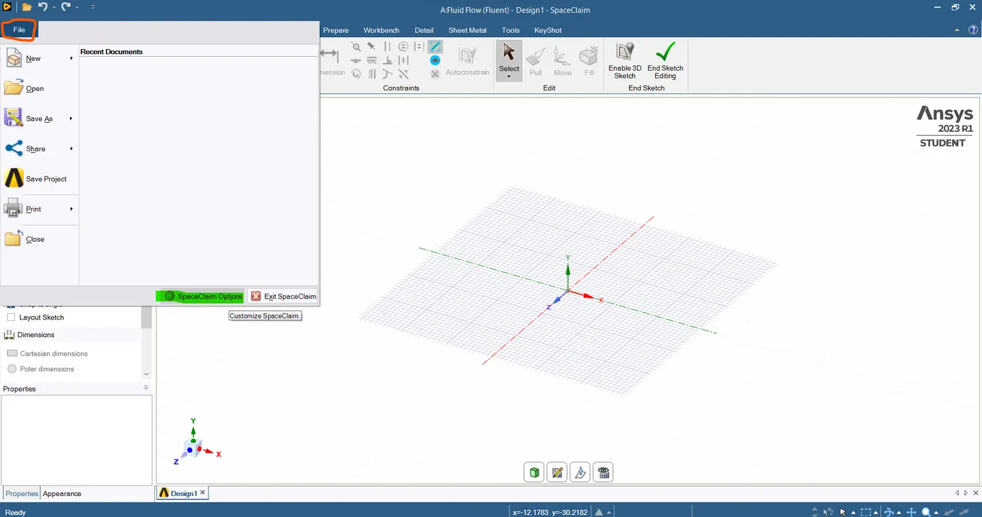
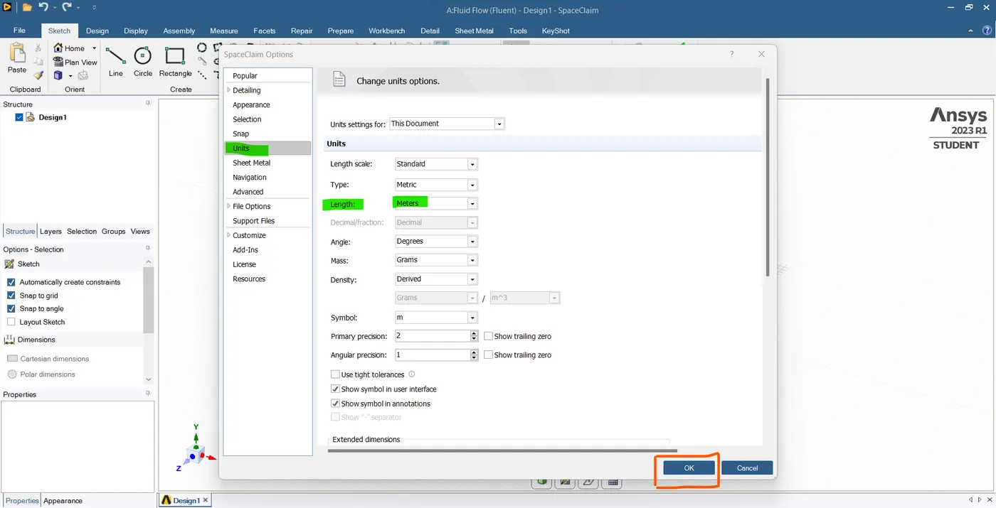
• Now we need to change the unit system measurements. so, go to the file option and then click on units the change the length into meters.
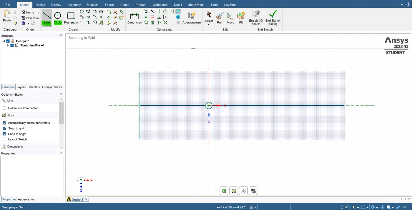
• Now we are going to start our sketch first start with our cylinder. so, in the design section. select the "circle" and enter the measure as 2 meters.

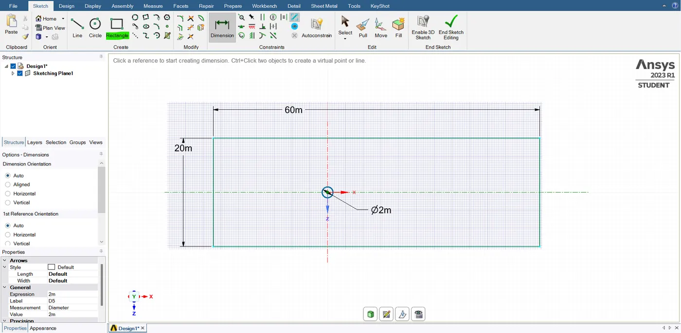
• Then we are going to create a rectangle computational domain. so as shown in the image we have to create a 20-meter line on the left side. so, select the line tool, and draw a line on the left side. now we have located the inlet correctly. 
• We need to create 20 times my diameter which is 40 meters. this is our location of outlet boundary. so, just create a 40-meter length line at the right side of my circle.
• we have to create a line at the side the length is 10 meters at top is 10 meters and the bottom is 10 meters. so, now once we created the line or once we have this we can create the rectangle box.
• so, basically using these particular corners and the kind of box we have to create. now we can see our rectangle box is created.
• And we can see the total length of my rectangle box. at the top of the box is 60 meter and both the left & right side of the box is 20 meter. so, it is perfectly got. Alright, that concludes our geometry-creating process. Since it's 2D so that's it's fairly easy.

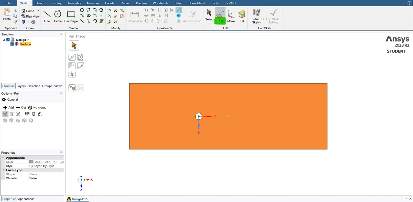
• now we have created our geomentry and need to convert this into the surface.
• so, in the design section just selects the "pull" tool, and after clicking that our geomentry. now instantly our geomentry is converted into a surface. it's changed the color. so, that means the surface that is created.

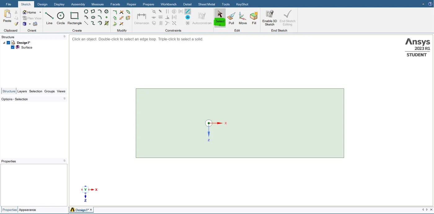
• Now after creating the surface we've to delete the circle inside our box. and then expand our curves to every construction line we have drawn. we can just right-click and delete so, that concludes the geomentry creation process.
• Make sure that the origin of the circle is the center of my circle it's very important. because we are going to add the monitor point. based upon this coordinate system.

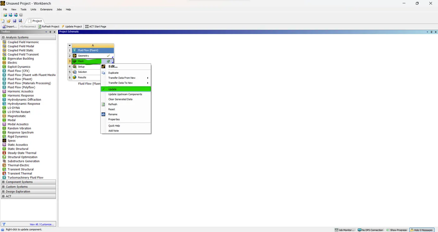
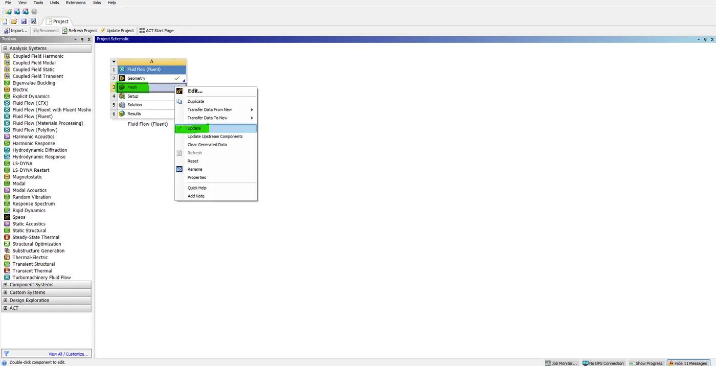
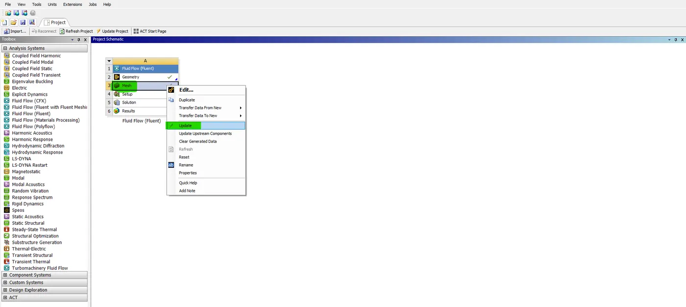
• Now just close this geomentry GUI. and right-click on mesh and click update. so, now our geomentry information is get's updated then double click on my mesh to open's our meshing interface.

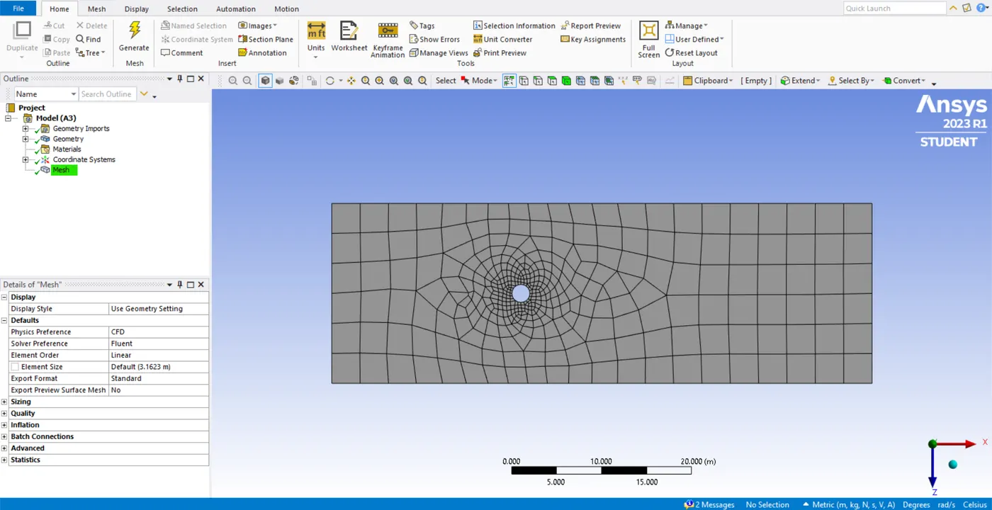
• after opening our mesh GUI. just click our mesh option on the left side. immediately we can see our mesh in our geomentry. it's called quadrilateral mesh or quad-dominant mesh. the quadrature contains 4 sides. so, we don't want this mesh. we need only triangular.

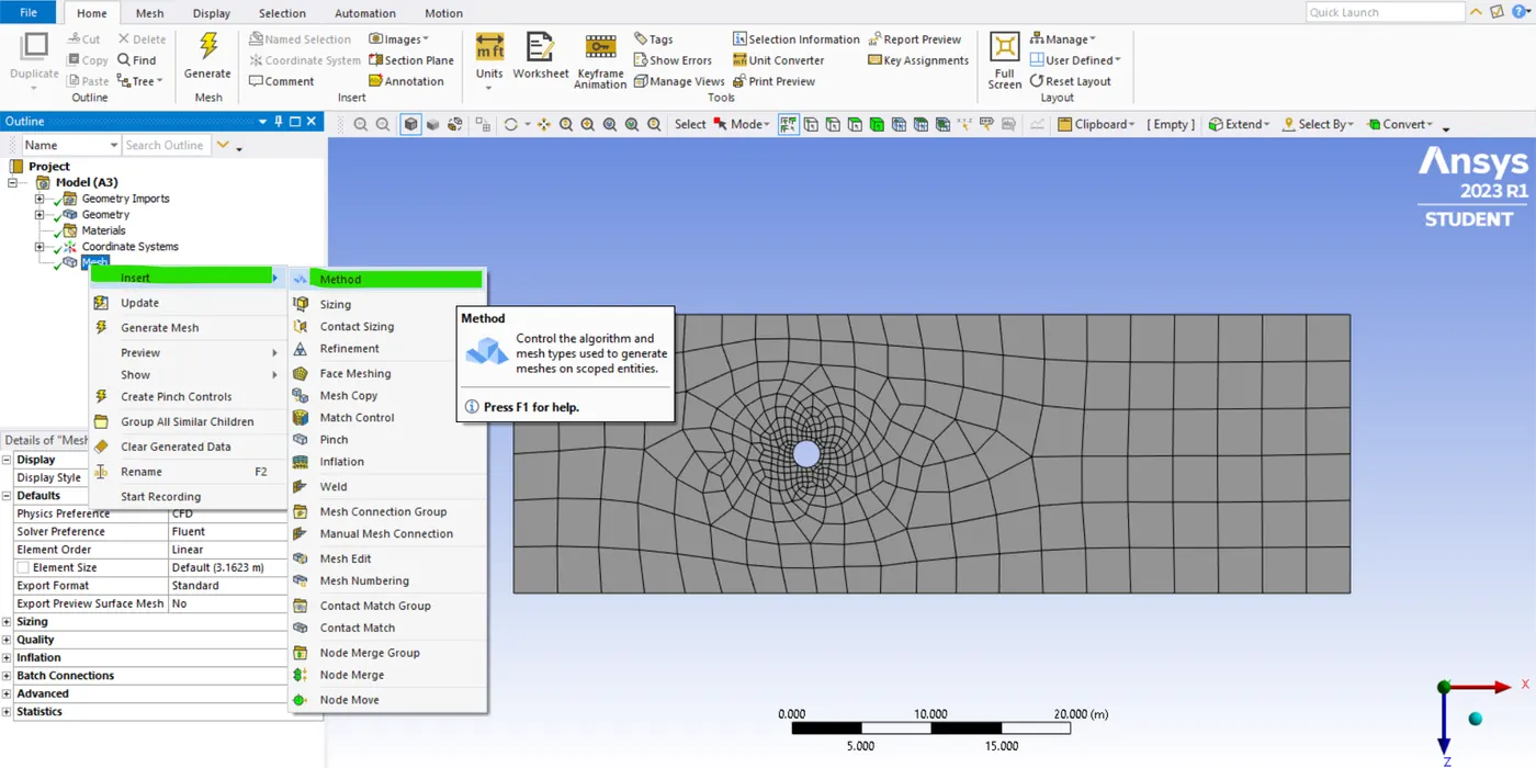
• so, just go to mesh -> Insert -> method. the idea is to add a baseline mesh and then we can add several methods.
• And the ansys is going to first create the baseline mesh and then it's going to include the method and just keep on processing our mesh the mesh that we added.

  

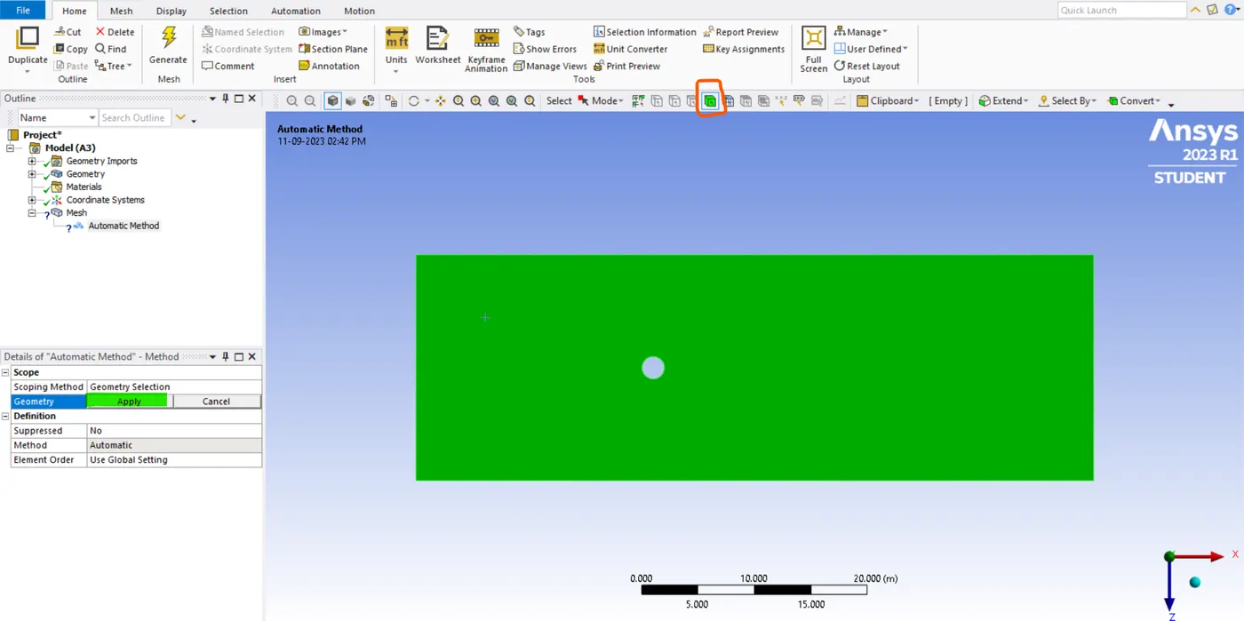
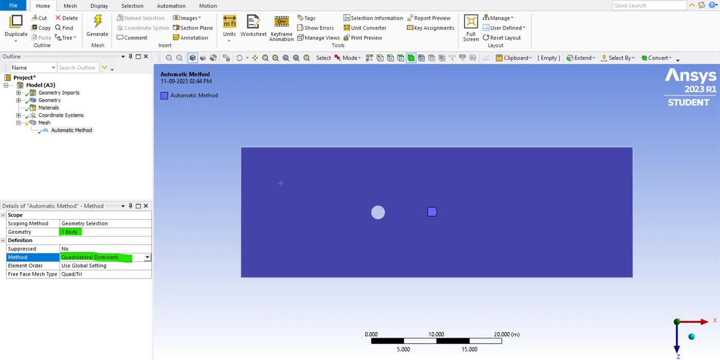
• Then we have to select the face in my geomentry. so, just go to the body option and then click our geomentry. now in our geomentry section just click apply and we can see in the geomentry section that there is 1 Body. Previously it was not showing but now after selecting the entire geomentry. it is showing that means it's saying 1 Body.

  

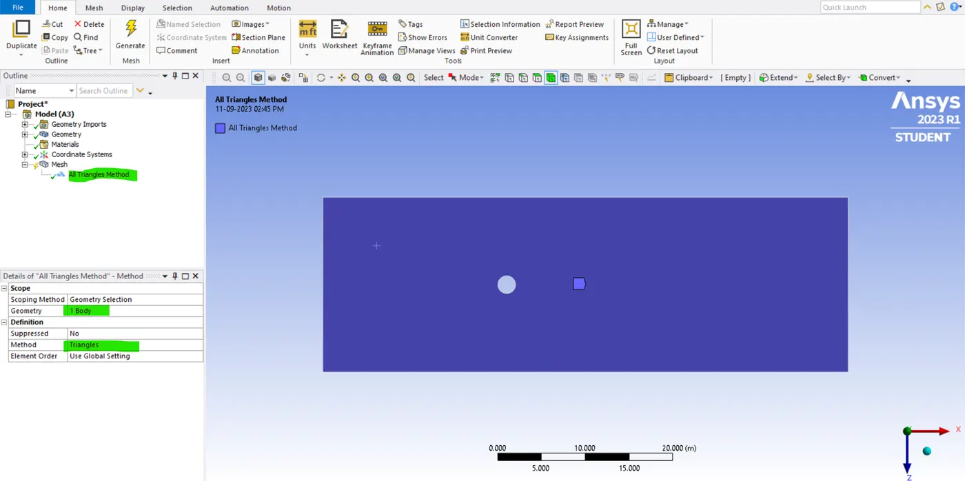
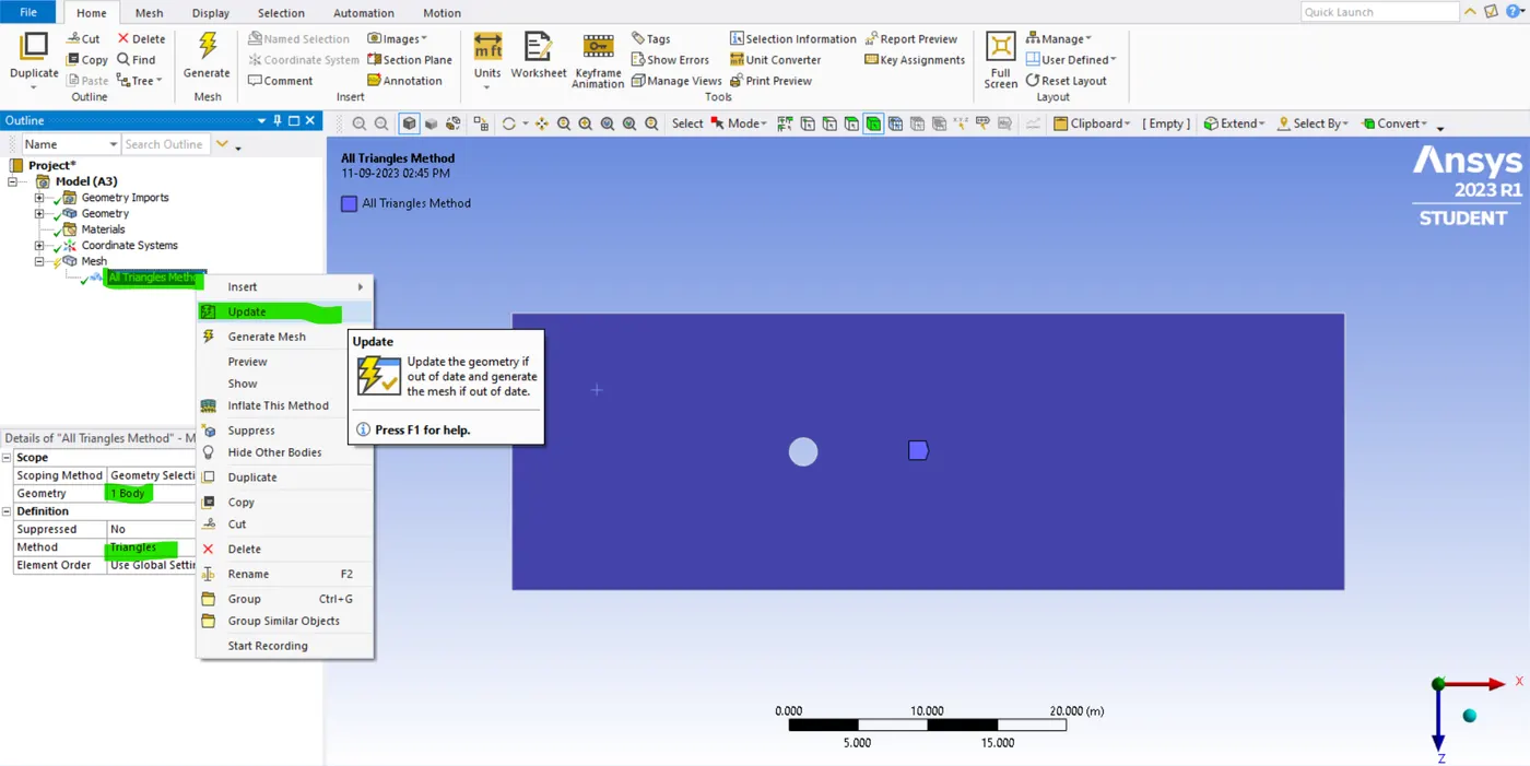
• Now we need to change our mesh type, so expand our default mesh method -> select triangle. Now click mesh and update or generate the mesh. and now we can see in our geometry the mesh is changed from quadrilateral to triangle. so, our mesh has been updated.

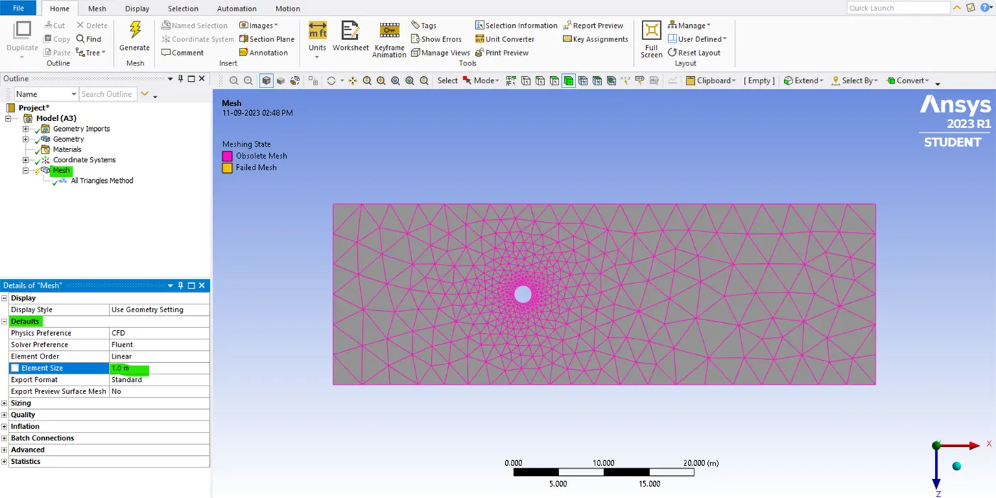
• Now we need to update our mesh size. so just go to element size and enter the value is 1 meter as my element size. now remember ansys is going to adaptively refine the mesh which is near the cylinder. and then after updating the mesh element valve, we have to update our mesh.

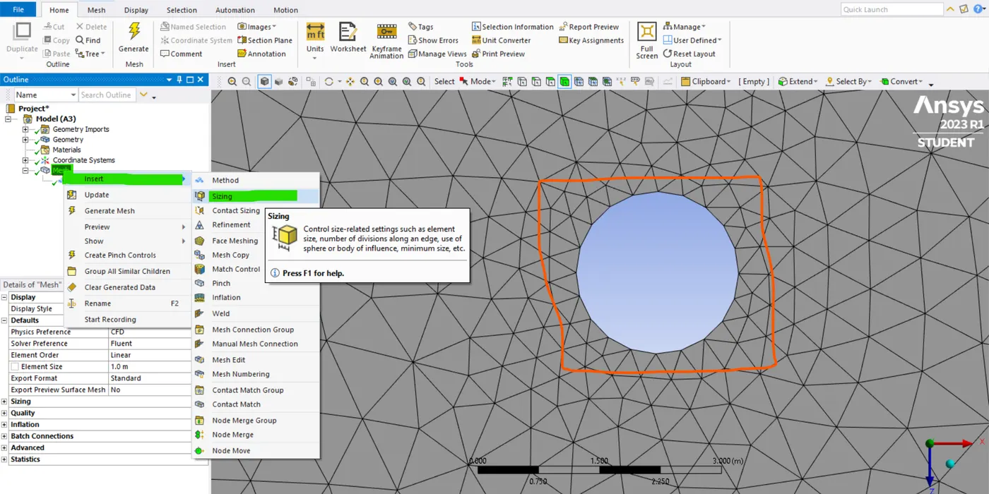
• In that cylinder that is in that circle it does not look exactly circle or it has a 12 or 13-face polygon. so, In that circle, many sharp corners will affect the flow field. 
• so, one thing we have to do in CFD is we want to make sure the geometry on top of which we simulate the flow is captured perfectly.
• so, just right-click on my mesh -> go insert -> sizing. so, this option is used to get presizeingly control the mesh. now just select the edge of the circle and apply. because the edge that you wanted to click applies.

 

 

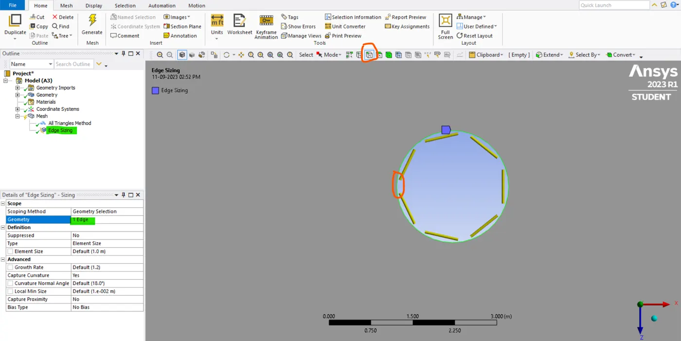
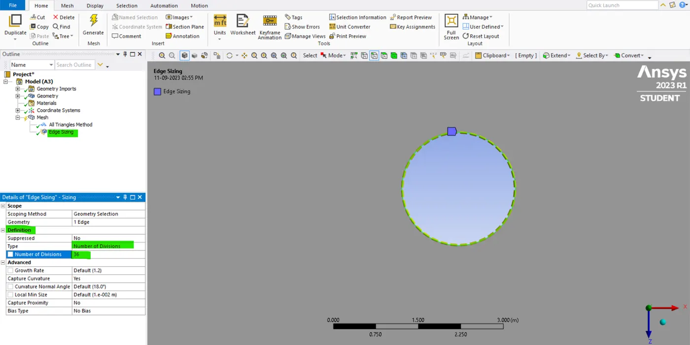
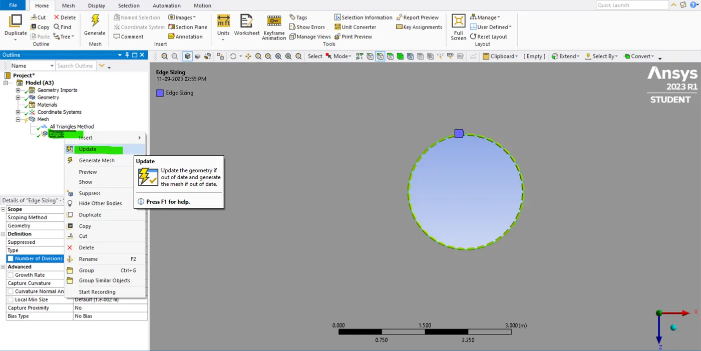
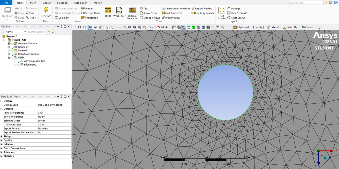
• And now we need to give the no.of.divisions. so, just go to type and select no.of.divisions enter the value in 36, and right-click on the edge sizing to click update. and now we can see after updating our edge sizing our circle edges are looking smoother than previously. 

 

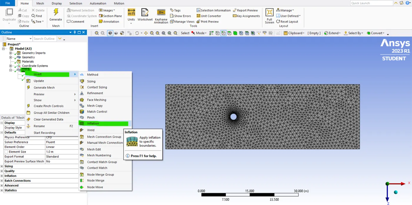
• Now once we want to make sure since the flow around. so, I want to take care of my edge region around the cylinder. and I can do this by selecting a mesh -> insert -> inflection option.

    

 

 

  

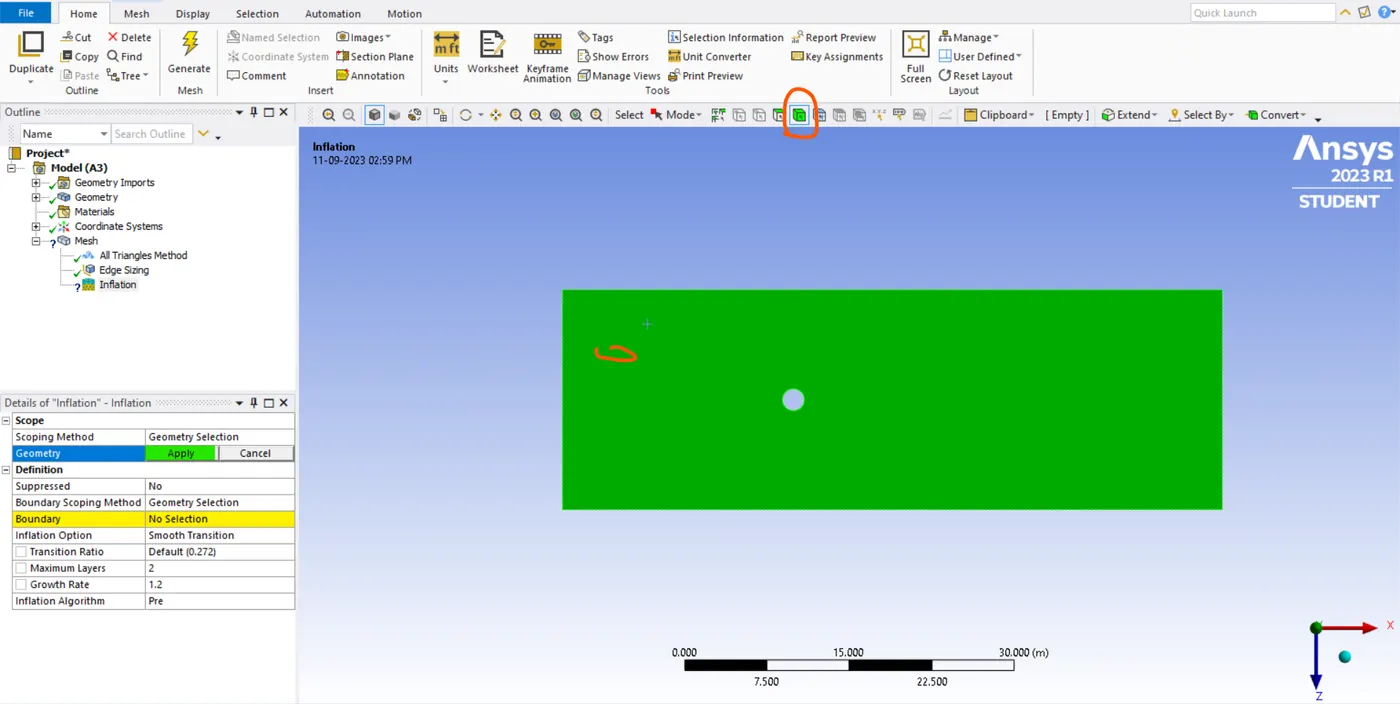
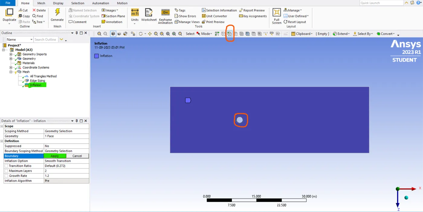
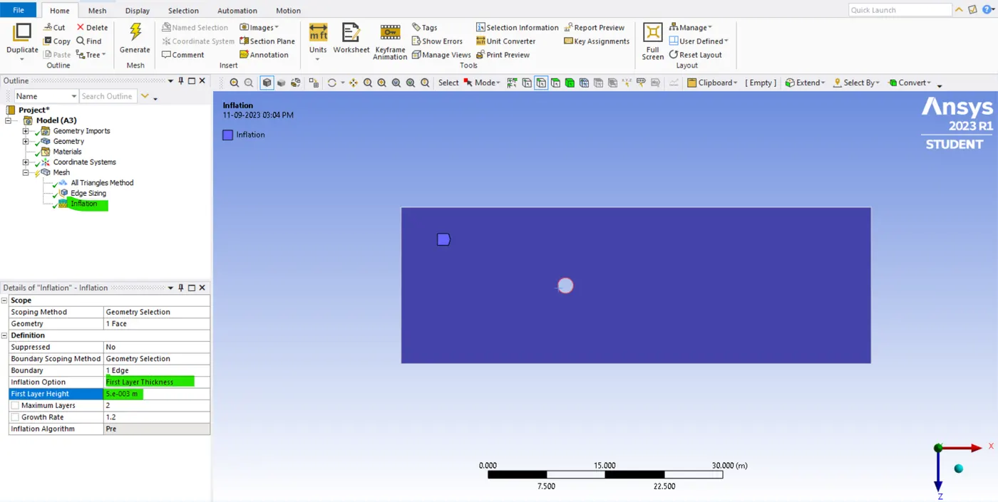
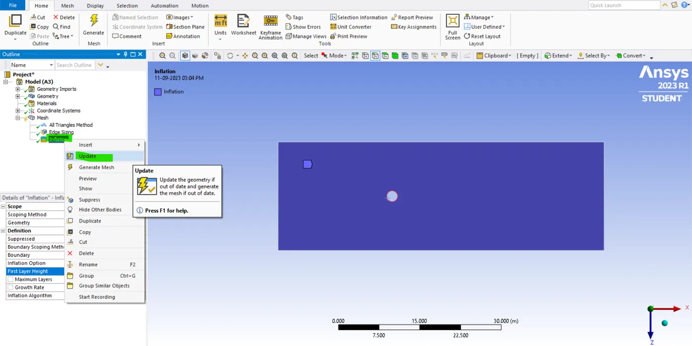
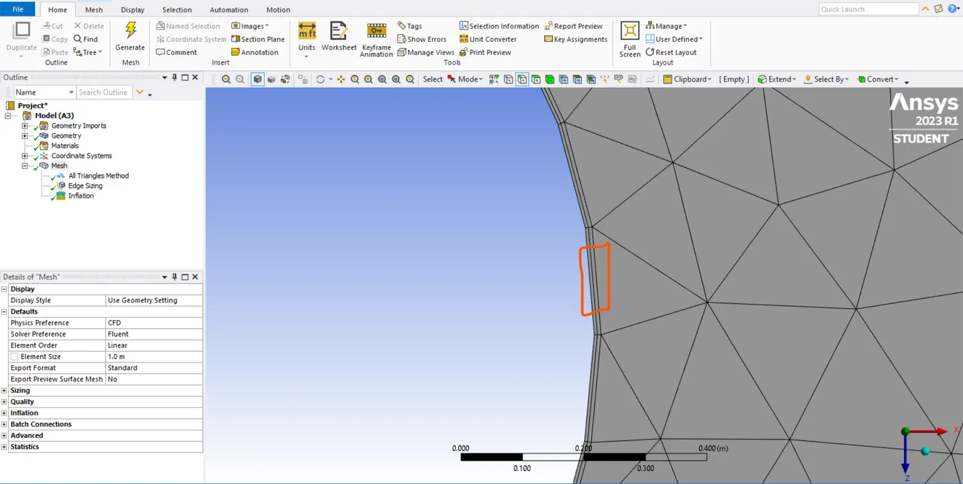
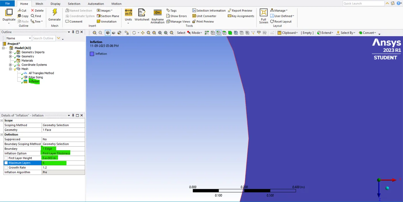
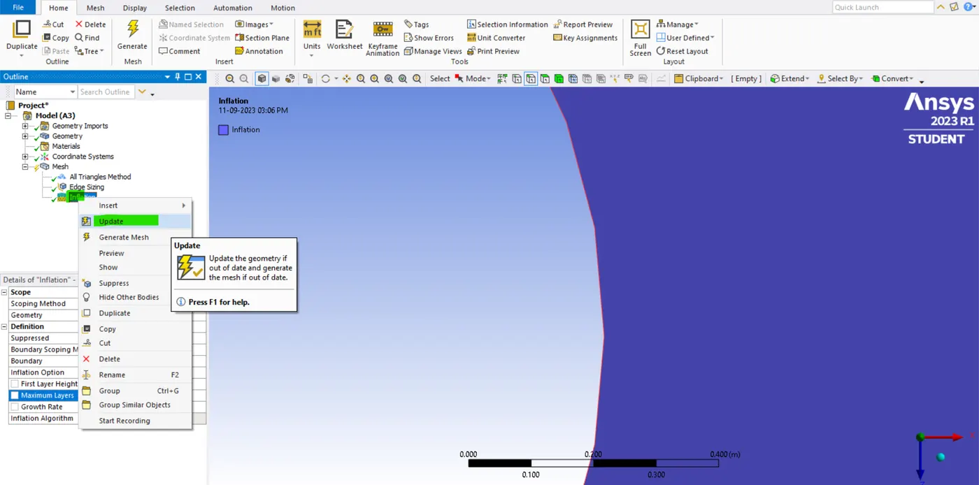
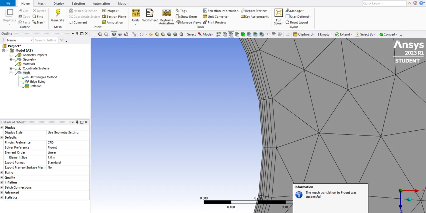
• so, the inflection layer helps to create a body-fitted mesh. First, select the entire face and click apply for boundary select this particular edge in our circle and apply. and select the inflection layer option-> first layer thickness. and our first thickness size is 5e-3. and then just click "generate mesh" or "update mesh". so, we can change the inflection layer max value is 6 and generate the mesh.
• Now we can see our inflection layer in our edge geomentry also we can see that closely followed in our geomentry. so, this is what we called as body fitted mesh the mesh fitted perfectly.
• So, the first layer looks exactly like a sphere. if you joined all the cell centers. if our shape is more like a square or ellipse and if we do body fit in. If we do it correctly then our mesh will represent our body very well that's why we called it body fitted.
• so, we added 6 inflection layers. so, we can see the initial cell size and the last cell size it's increasing our inflection layer cell site gradually. and that's because the growth rate factor is 1.2. so, it is a 20% growth rate. The first inflection layer is 5mm and the second layer is bigger than the first it's increased by 20%. so, till the 6th layer, it gradually increases and ends. 
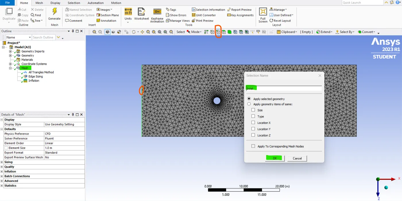
• open mesh GUI once and we need to assign the inlet and outlet names. For this just go to edge selection and select the left side of the rectangle and we can use the shortcut "N" or right-click that and create a name selection and give the name "Inlet".

  

 

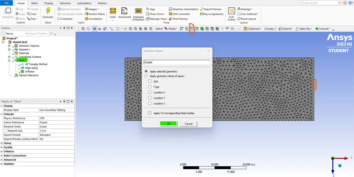
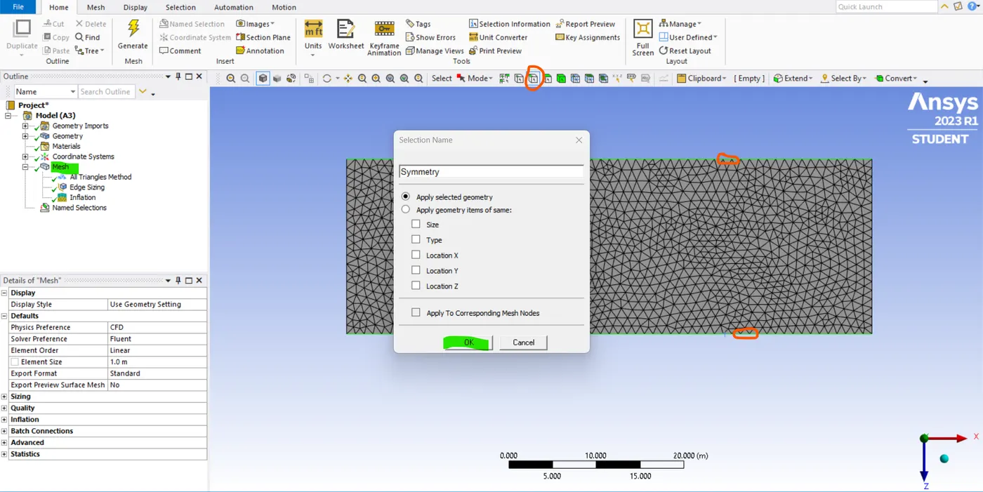
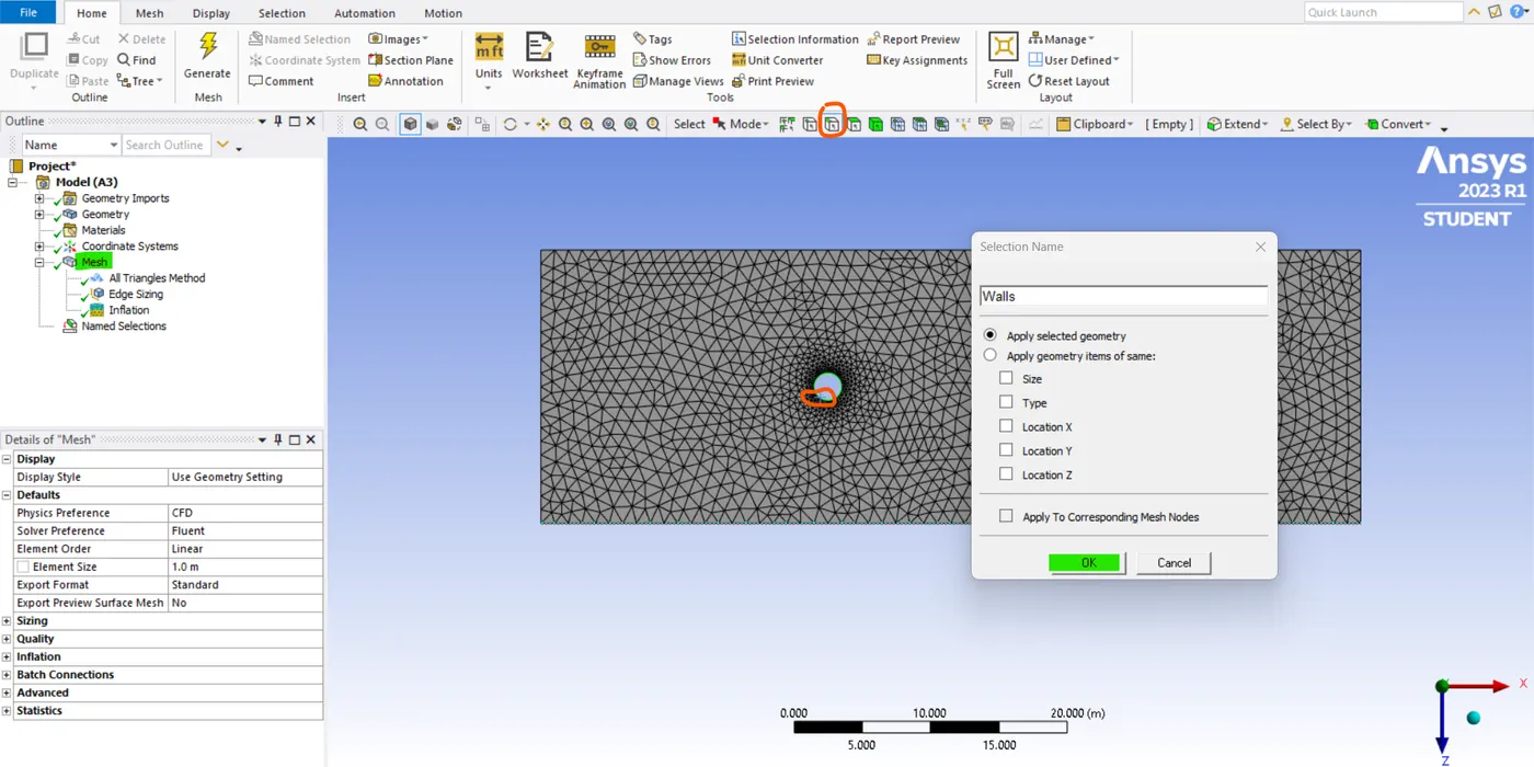
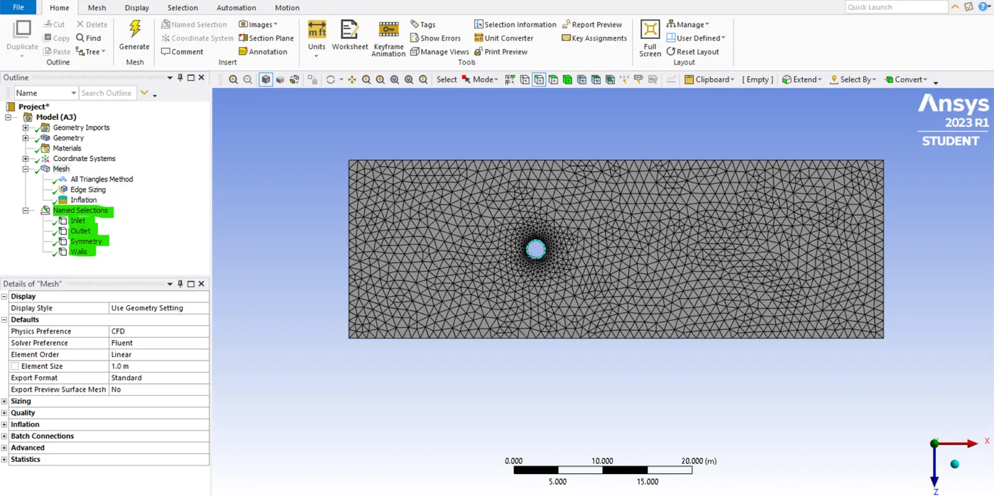
• At parallel on the other side use the "outlet". at cylinder edges assign the name "cylinder wall". and the top and "symmetry" close this mesh GUI and update it.

2. Solving(setup, solving) :-

  

  

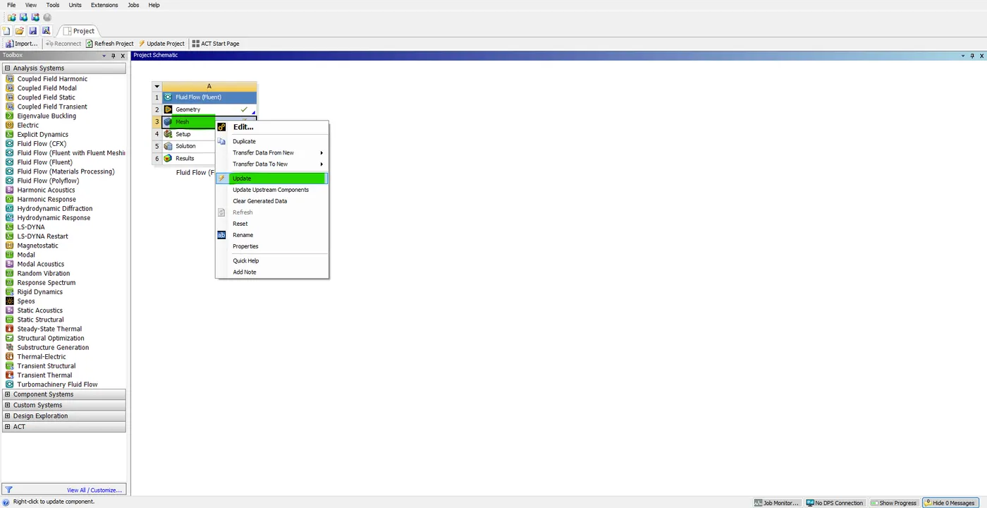
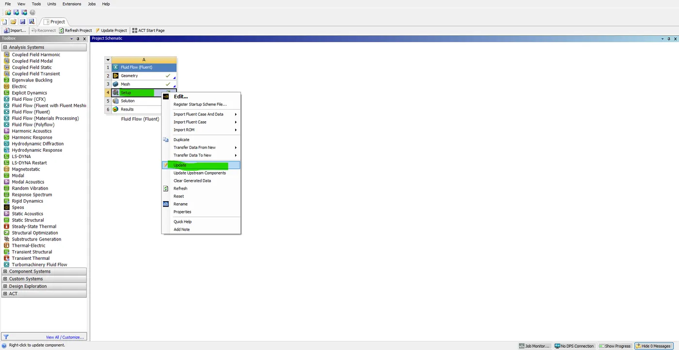
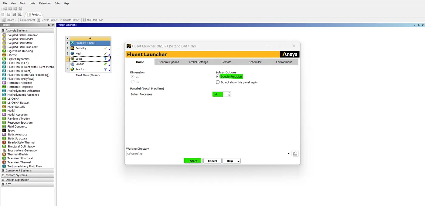
• so, Now let's close this much GUI and open the setup GUI before opening the setup just update the mesh once. After opening the setup GUI we need to check the boundary conditions. so, that means it has been loaded to the setup.

  

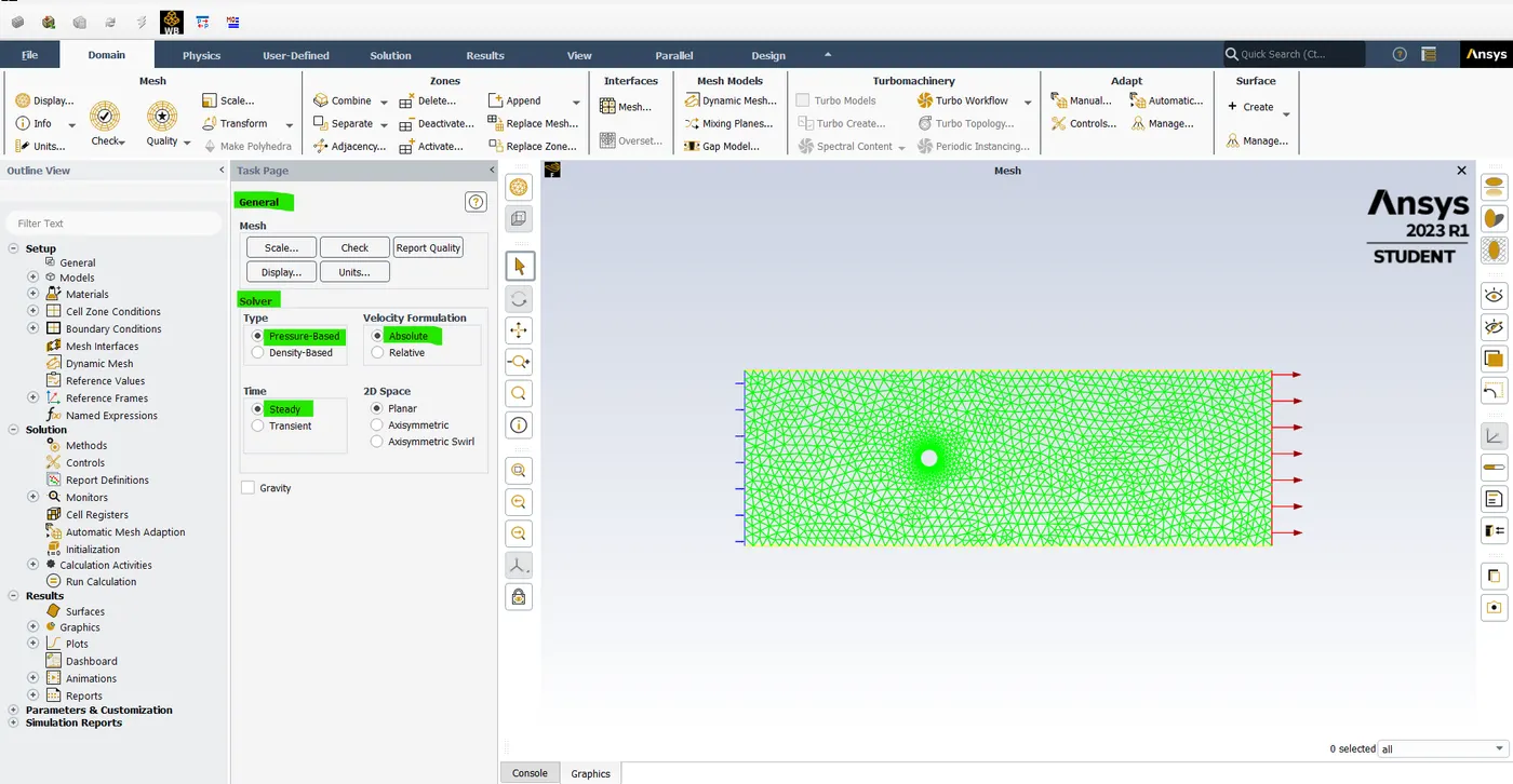
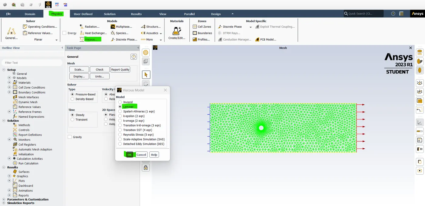
• now next thing we need to check the solver. so, here we are using the "steady state" in time and "pressure based" type, and "absolute" is a velocity formation. and then click on viscous model choose the laminar and click OK.
• Here the viscous model is laminar the reason why we are doing this is because our Reynolds number is going up to 100. which is a completely laminar region.

  

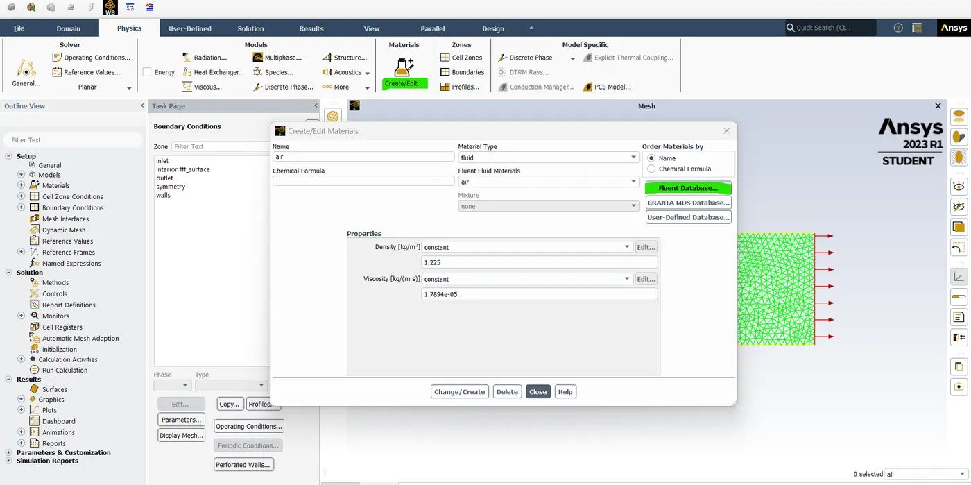
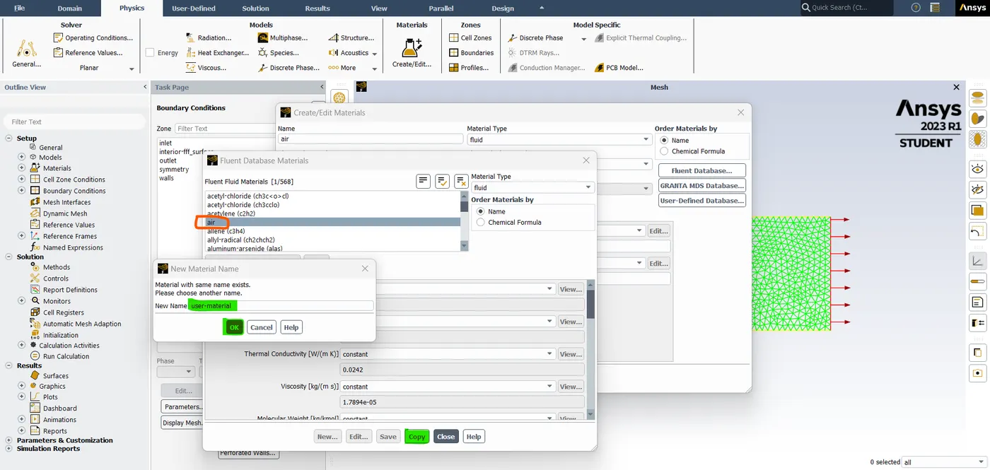
• the way I'm controlling the Reynolds number is by modifying the dynamic viscosity. so, let me click on Create and edit in the materials area. and then click the fluent database in that select air and then click copy. now we need to define the material name as "user-material". so, we created the customized fluid, and let's "ok" and close this tab.

   

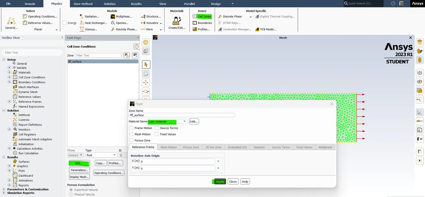
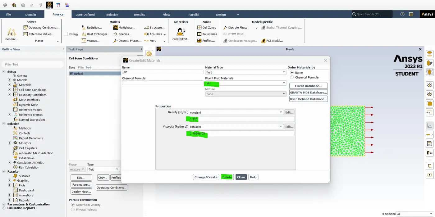
• So, now we need to select unwanted material and then delete that material. if it is not deleting just open the "cell zone" and then select open the FFF_Surface change the material name into user-material and click "ok". 

  

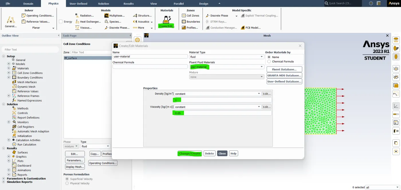
• Now go back to the material and then delete the air material select the user material and click "OK". And then we need to change the density and velocity. so the density is constant and the value is 1. And my viscosity is constant and at 0.05 Kg/ms click "change and create" and "close".
• so, the reason behind this vicious value is that in this condition it has been documented that we start seeing the vertex shading even in laminar flow conditions and this is what we call a "Von Karman vortex street".

  

  

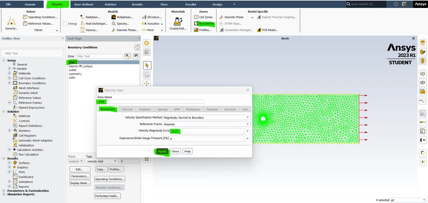
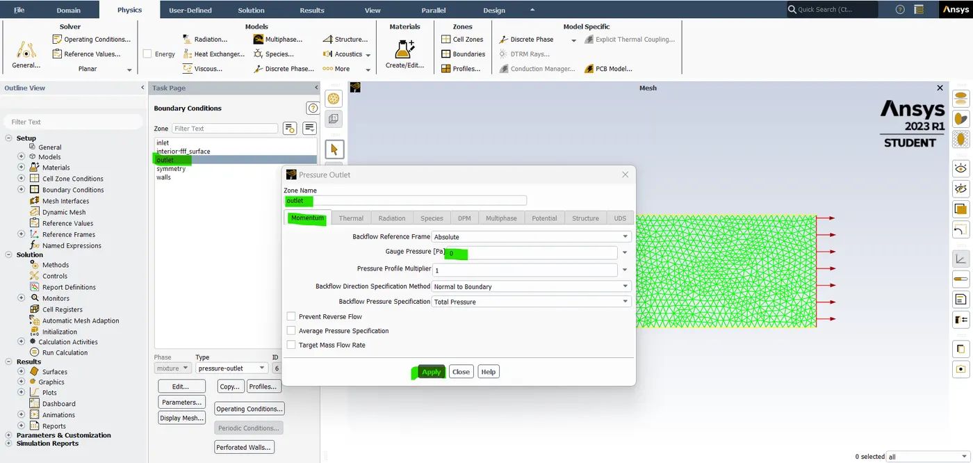
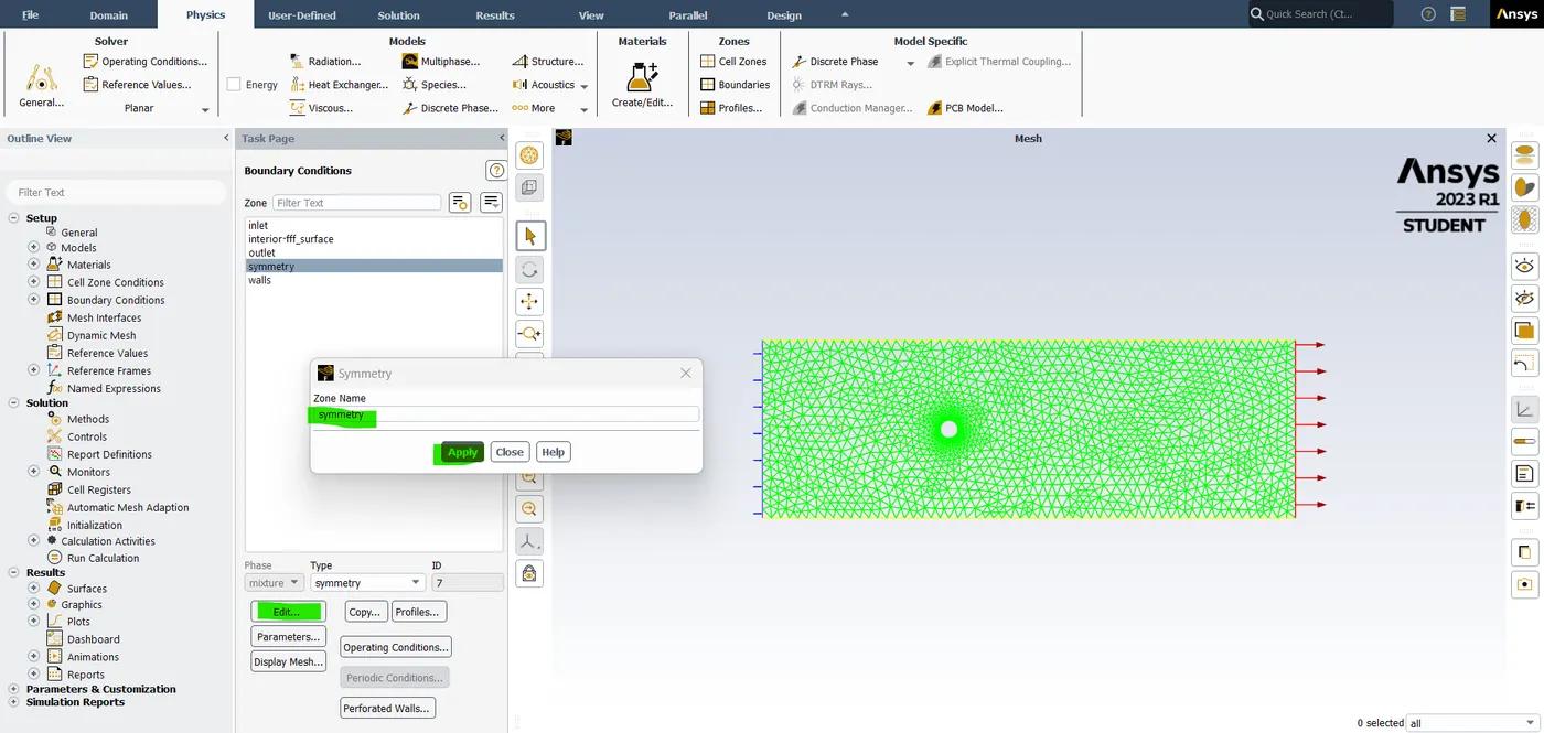
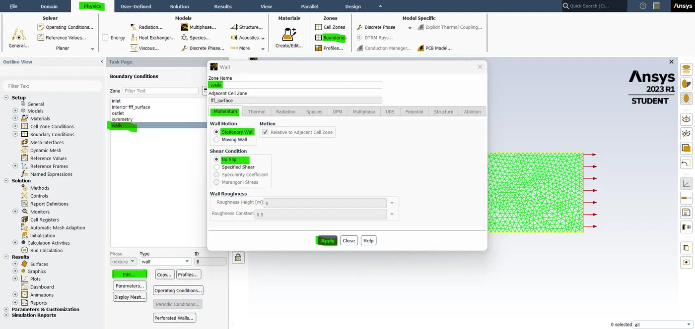
• Now we need to set our boundary conditions the inlet velocity is 1m/s. The outlet velocity is 0. and for the wall, we just make sure that the momentum of wall motion is "stationary wall" and the shear condition is "No slip" and click "OK". 
• For the cylinder we use no-slip condition meaning the first cell that is attached to our cylinder and the velocity is zero. the symmetry is automatically assigned as a symmetry.
• the next thing we need to do is to look at the different flow quantities. while the solution is being generated. so, for that, we are going to use a "definitions" option.

     

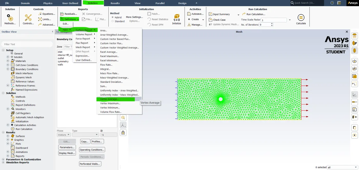
• so, click "Definition" -> New -> surface report -> vertex Average. in the name, section enter the name as a monitor point. and then we need to select the monitor point, but there are no monitor points here. so, just close this tab.
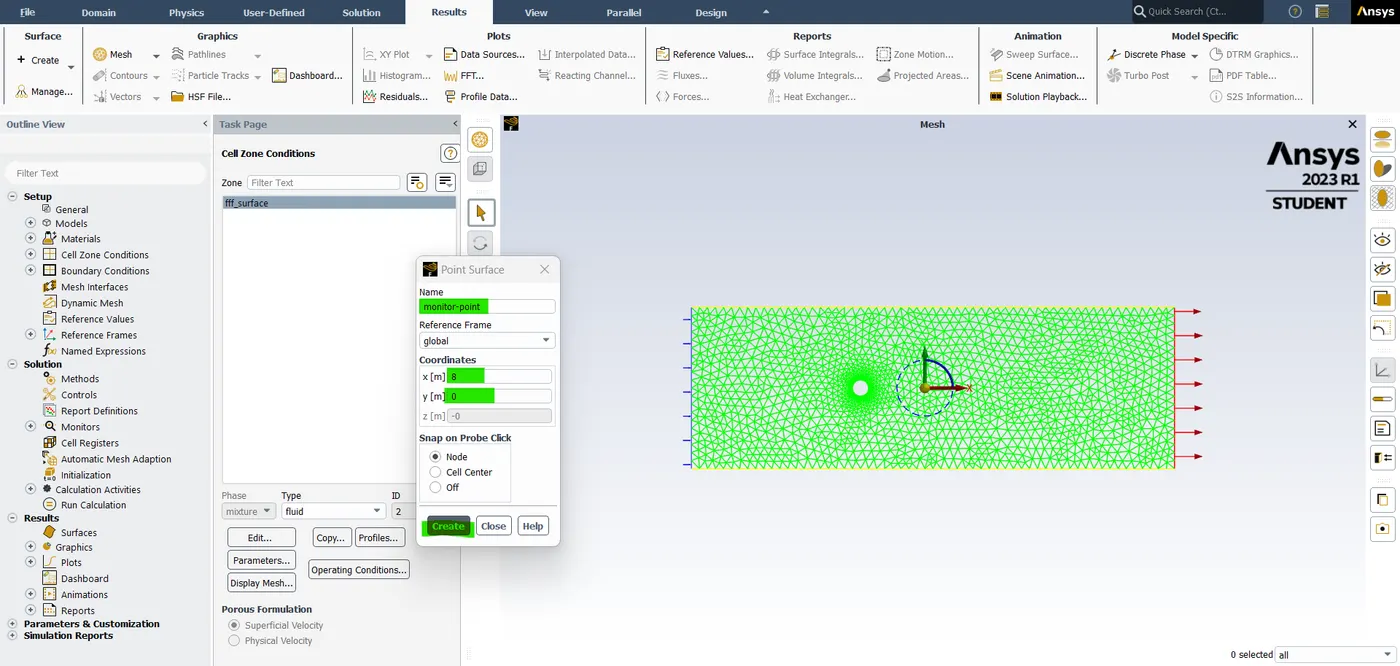
• so, go to the postprocessing section and select the "point" into a create option in the surface section. so, after selecting the point we need to create a point at 4 times the diameter which is 8 meters.
• In that point surface tabe enter the x-value as 8 and the y-value as 0. and the name of the surface is monitor point and then just click the create and close.
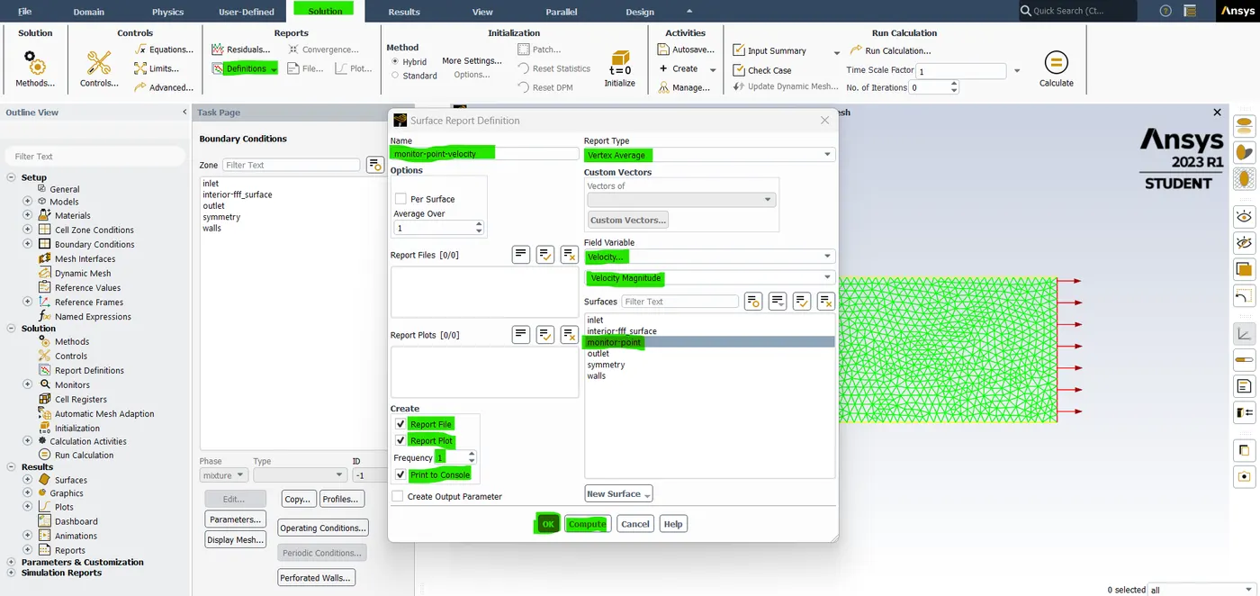
• Now we have to go back to the solving and definition -> New -> surface report -> vertex average. after opening the report definition name as a "monitor point velocity". Select the monitor point and select the field variable as a velocity and velocity magnitude. so, we are going to see the vertex average into our monitor point click on the report file plot, and print to the console and the frequency rate is 1.

  

 

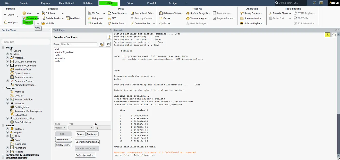
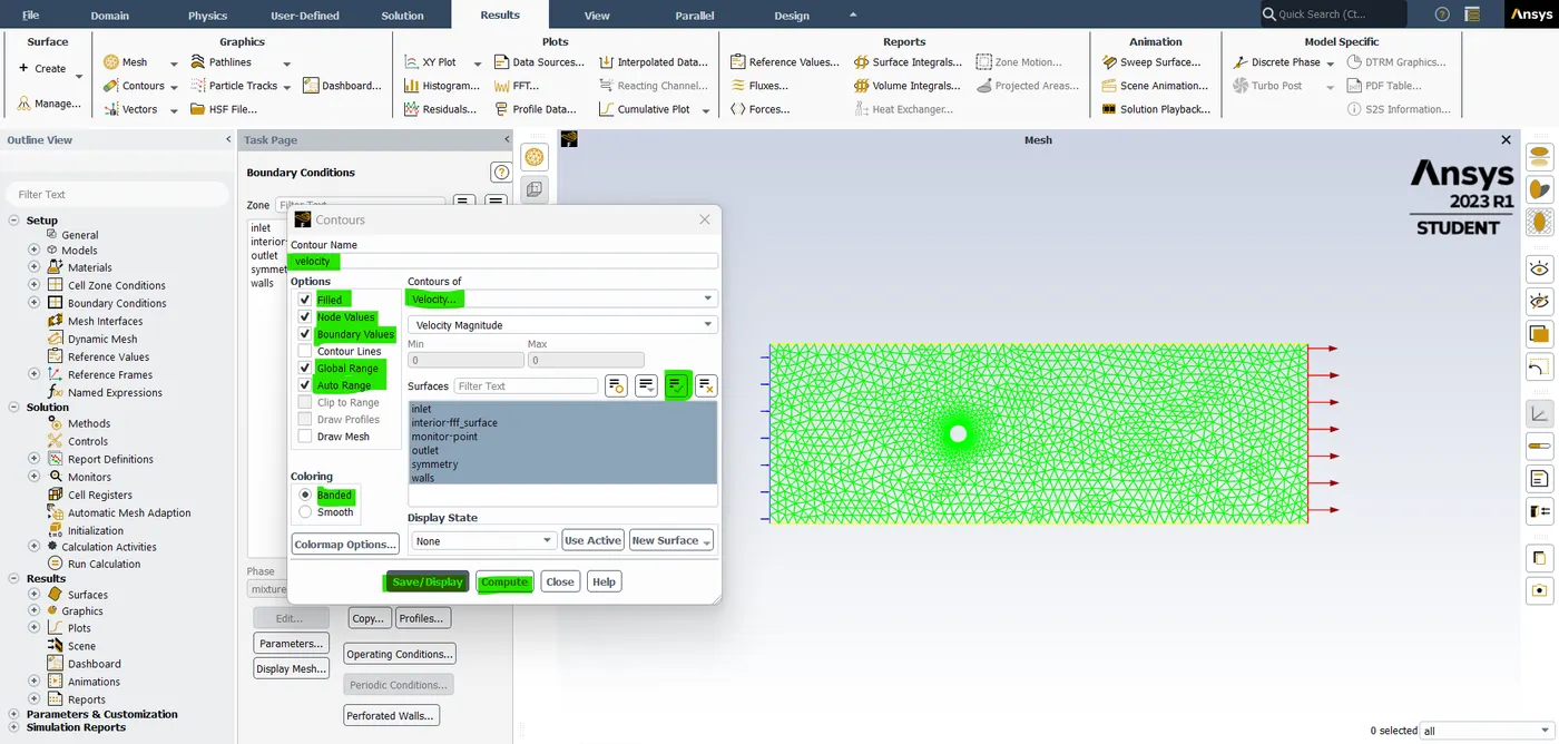
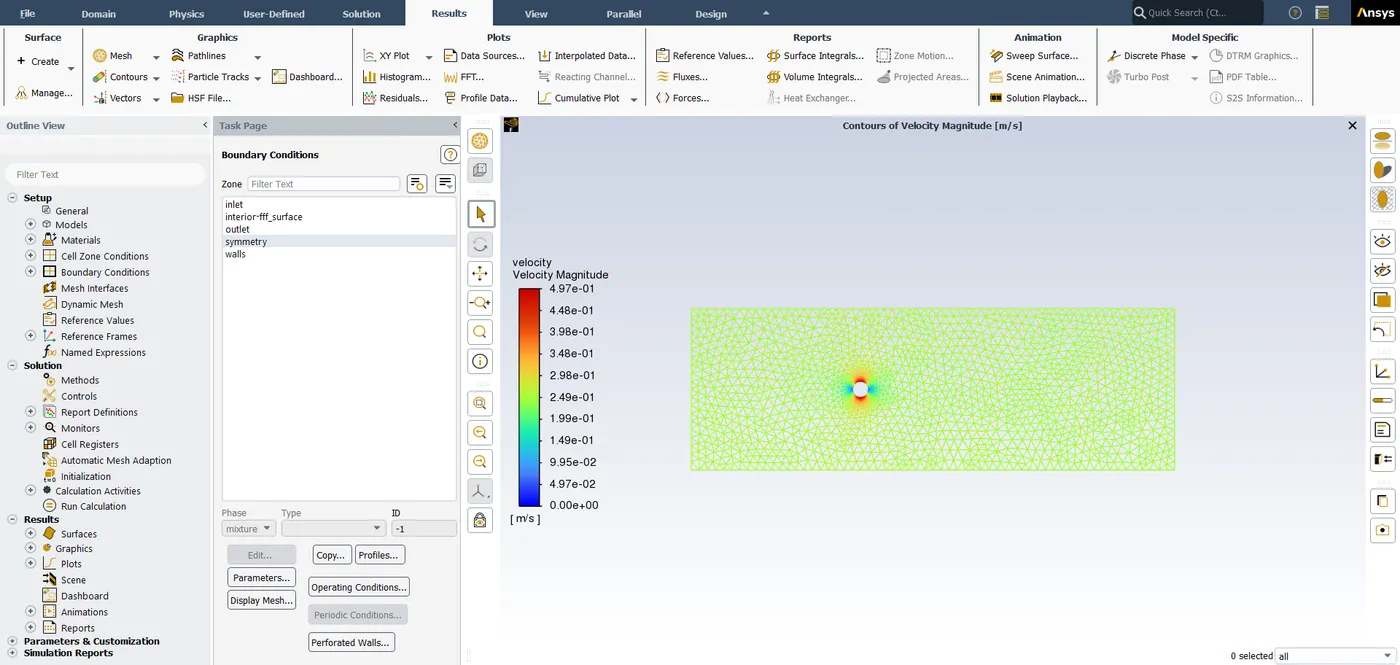
• In addition we want to create a velocity plot and pressure plot. so, these are the contour plots. so, to do that we have to initialize a hybrid initialization. so, now our domain contains some initial value of velocities with which we can set up our contours plot.
• go to post-process and select contour -> new option -> name as velocity -> contour of velocity -> make sure select boundary conditions -> click on save/display and compute. 
• Now go to our graphics screen we can see the initial value in our screen that was obtained by a hybrid initialization and it's not a final solution. so, just close the contour tab.

  

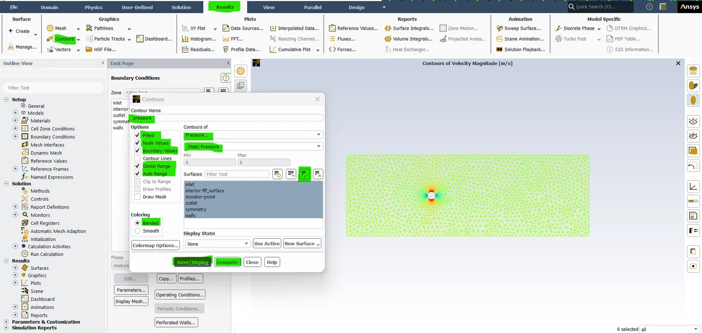
• so Anthen now we have to create a  pressure plot. so, go to Contours -> New -> Name as a pressure -> Contour of pressure -> make sure to select the entire boundary conditions -> click on save and display and compute and close the tab.

 

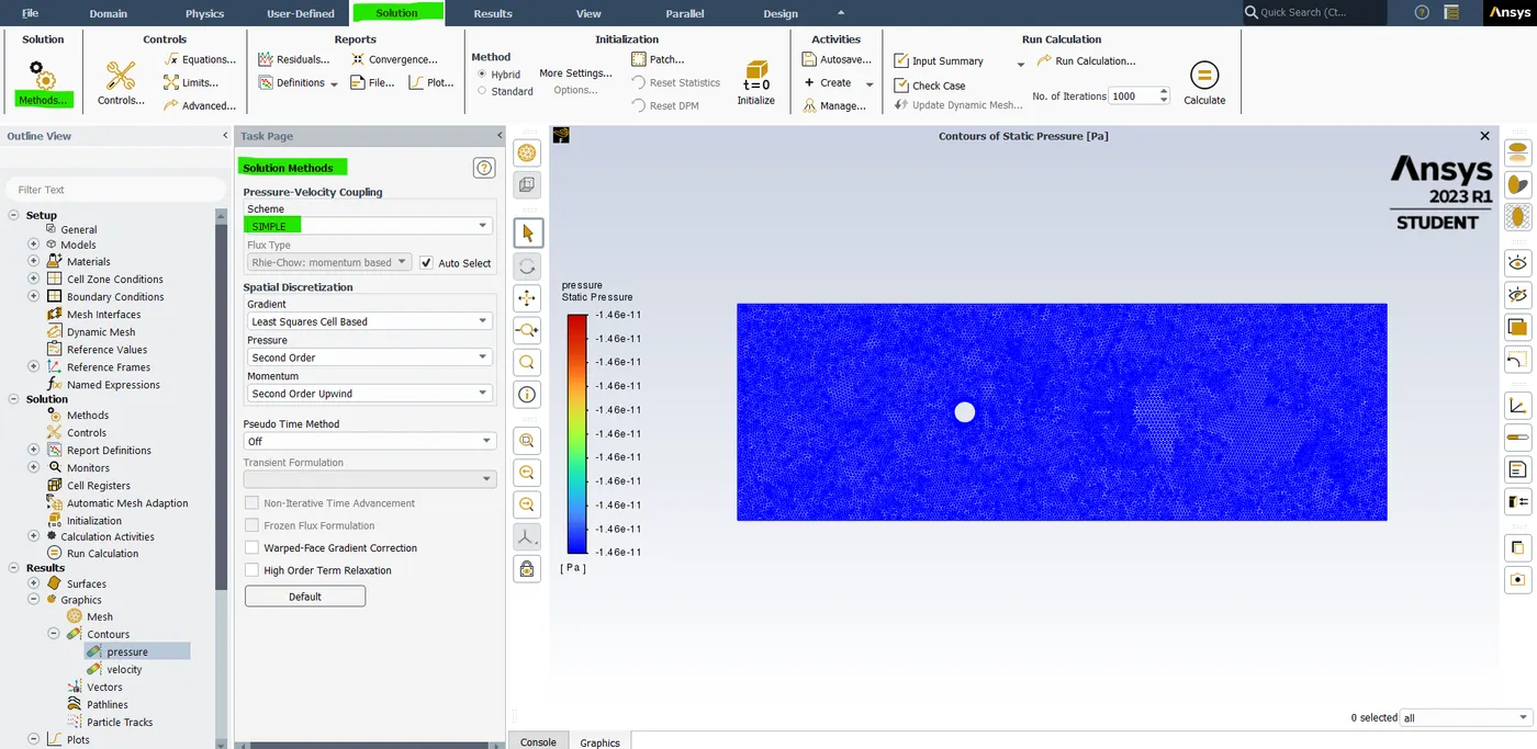
• So we created the contour plot and we have to go back to our "solving" section. so, click on solution and we are using a simple scheme solution, and click residuals in the reports section.

  

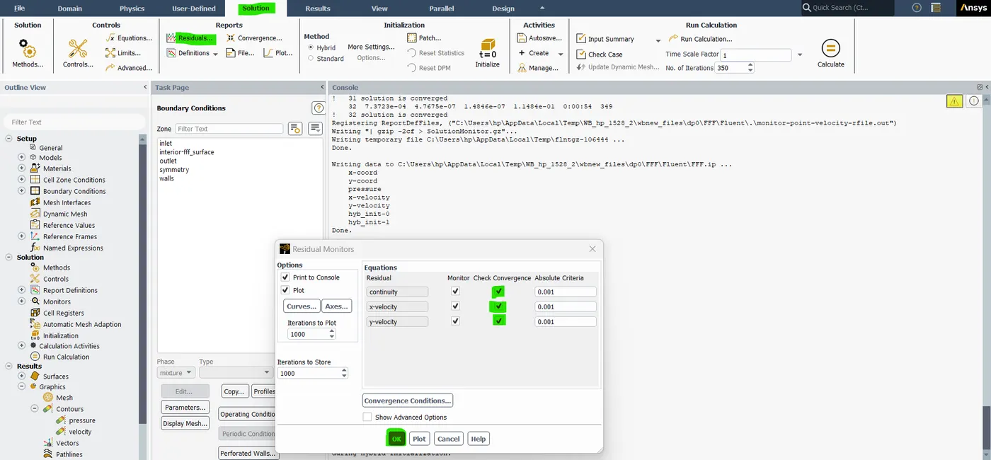
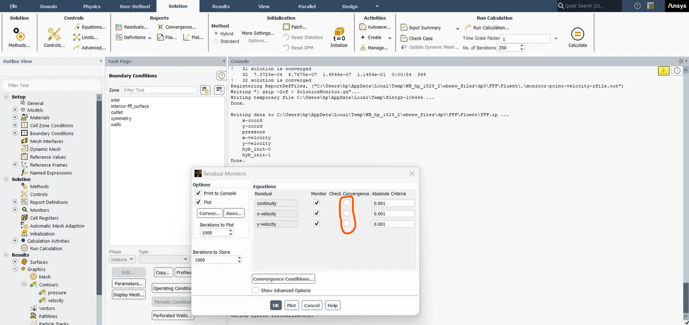
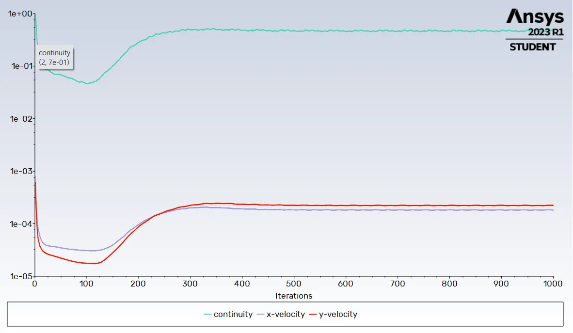
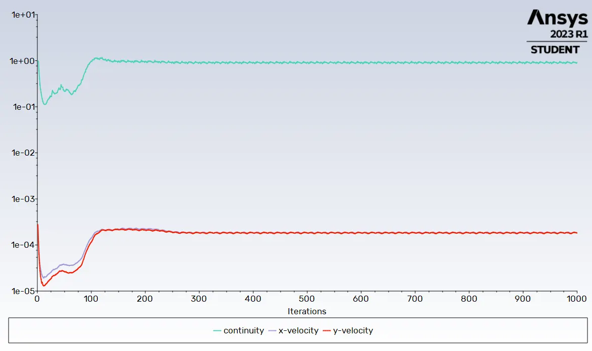
• so, In Residuals, we are looking for continuity and x-velocity and y-velocity. so, the x and y velocities represented the Residuals From the x-momentum and y momentum equation and now we have to uncheck the continuity and x-velocity and y-velocity converging criteria and click on "OK".
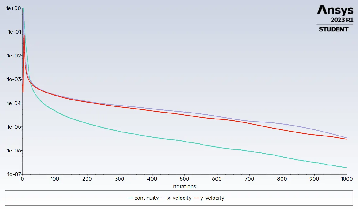
• so, the reason we did it unchecked is that we wanted to see the solution till the No. of. iterations that we gave the input Sometimes we entered a large No. of. iterations. but the solution will stop much before that and sometimes that is not very good. because it cause be that the physics in our problem takes a little bit of time to evolve and in the initial phases not happen.
• so things converge very quickly and the fluent might think that this is a final solution. so, we don't like that so, that's why we are providing a manual no.of.iteration. sometimes this also doesn't work.
• it's always important to make sure that the solutions are converged.

  

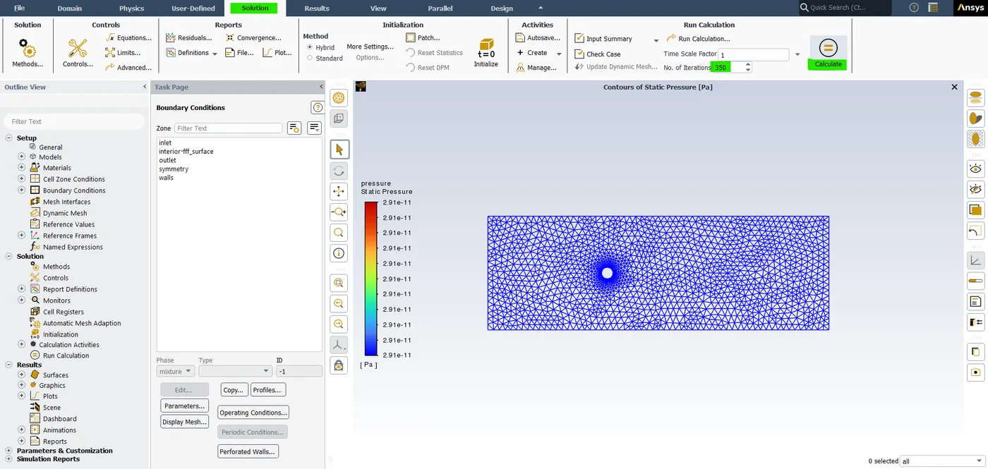
• Now after entering the no.of.iterations hit the calculate button. we can see our scaled residuals and our monitor point velocity report. after the 120 iterations, no changes are happening.
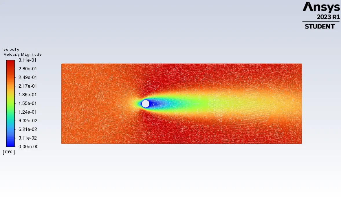
• On the left-hand side click the velocity and pressure contour in the result section we can see the velocity plot so, there is no vertex shedding happening. that means our velocity line is not fluctuating.

   

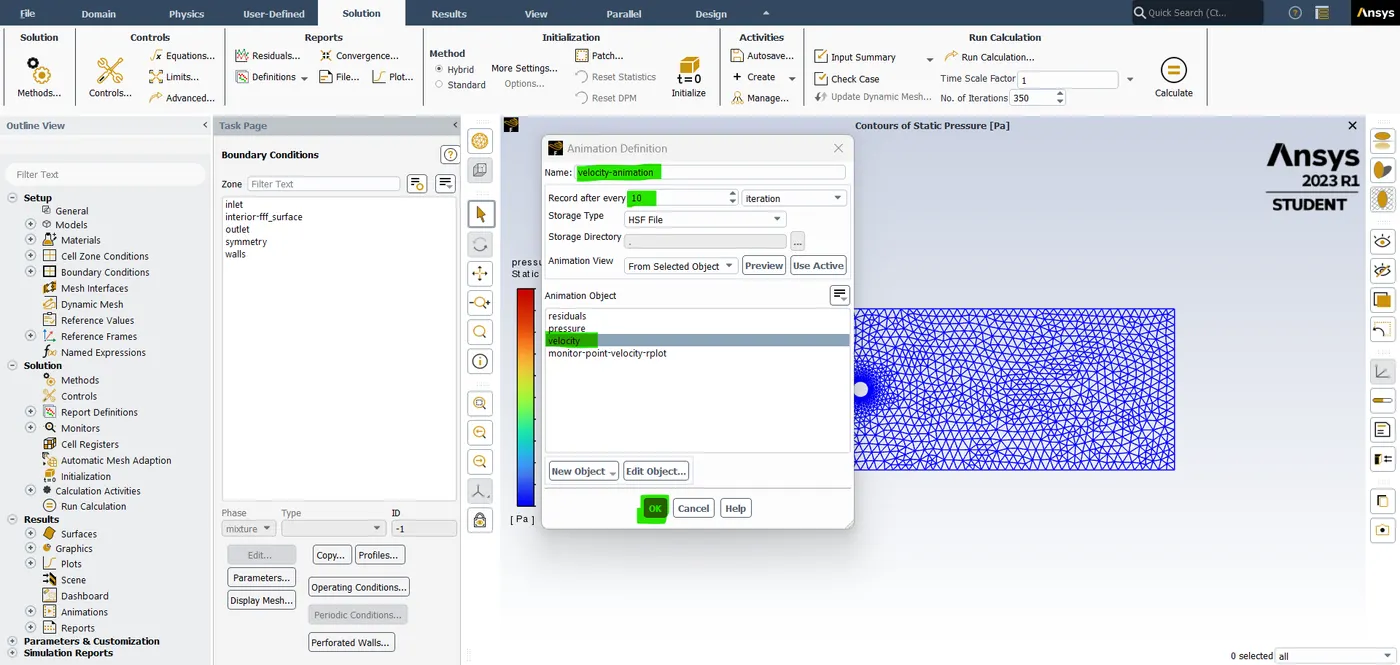
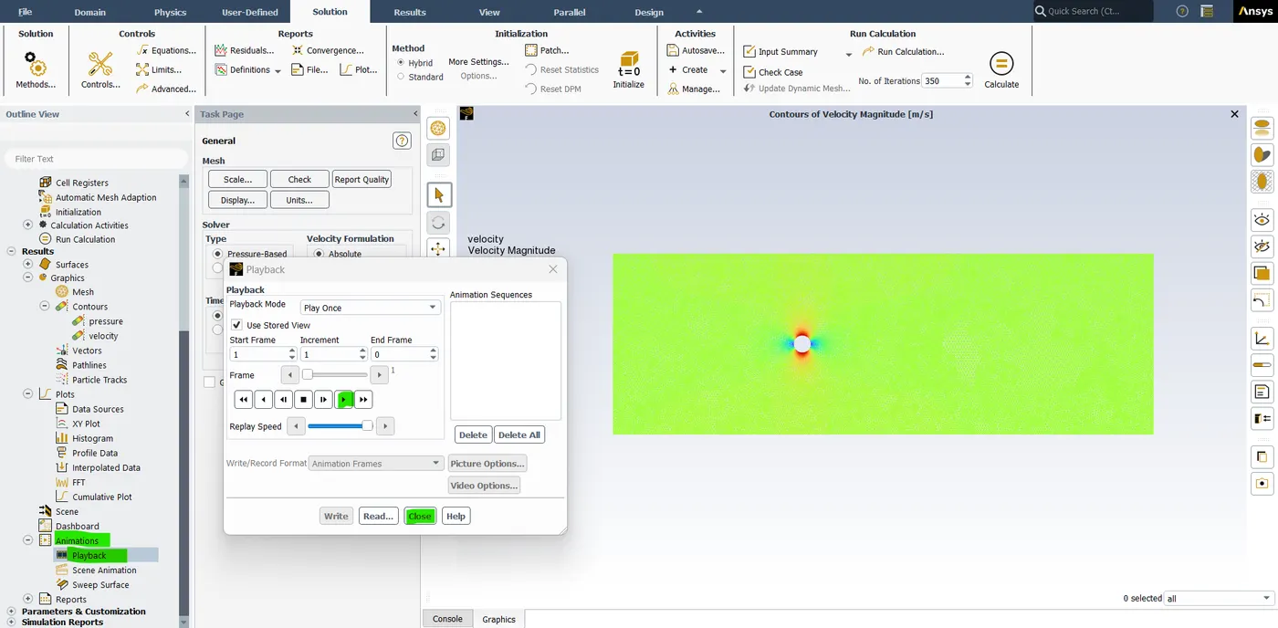
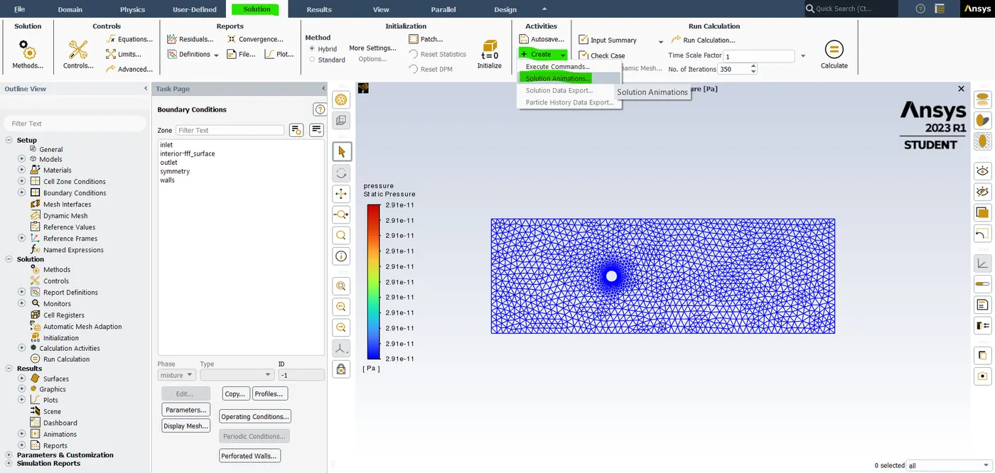
• so, one thing we have to make sure the solution is going to change the function of iteration it might be a good idea to add some animations. so, go to activities section -> click on create -> solution animations -> named as a velocity animation -> record after every 10 iteration -> select the velocity -> click "OK".
• so, To see the velocity animation we need to initialize one more time and hit the calculate button. after completing a calculation we can see our velocity animation in an animation area -> solution animation playback -> edit -> click the play icon. now we can see the changes in the flow of the velocity and hit in the close.

• so, in that video animation solution there are no any vertex shedding or fluctuating line changes. so, it is kind of bad we did obtain a solution but it did not simulate the physics that we are looking for. now we know for sure when the Reynolds number is close to 40 or above 40 we are supposed to start seeing the "Von Karman vortex shedding".
• so, click the create / edit. button in setting up physics changes the velocity from 0.05 to 0.045. so, it looks everything like is correct. so, we need to reduce the mesh size. so, close this setup and open the meshing interface.

  

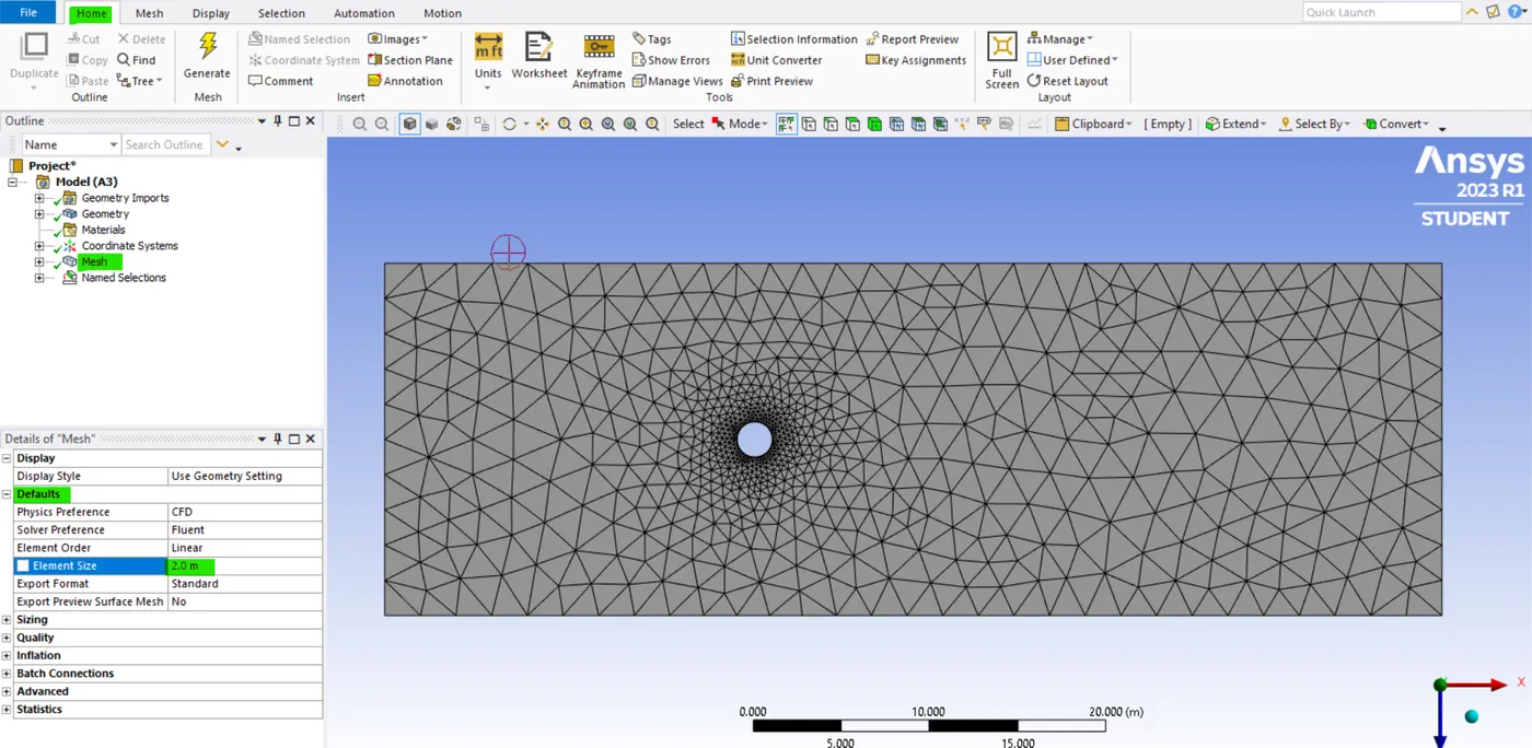
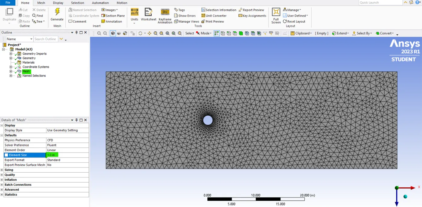
• so, open the computational mesh. so, now I'm just going to do it under the mesh parameter from 2 meters to 1 meter.
• so, we will see if that helps out if it doesn't we have to come back and refine it further. so, we have our base mesh and inflection layer and all the stuff right now. so, this is good now let's close this mesh GUI . and open the setup GUI.

  

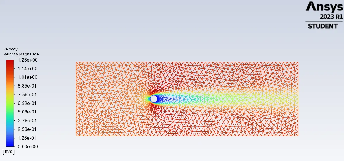
• so, before opening the setup GUI we have to just update the mesh and the setup block. so, after updating the both mesh and the setup block open the setup block alone.
• so, re-initialize everything one more time enter the no.of.iteration as 350, and hit the calculate button. so, we can see the behavior still seems to be the same there is no difference okay. so, we have to go to look at the animation as well to see if I can see some kind of vertex shading. and this is nothing here. so, that's bad. so, let's close this setup and refine our computational mesh one more time.

   

   

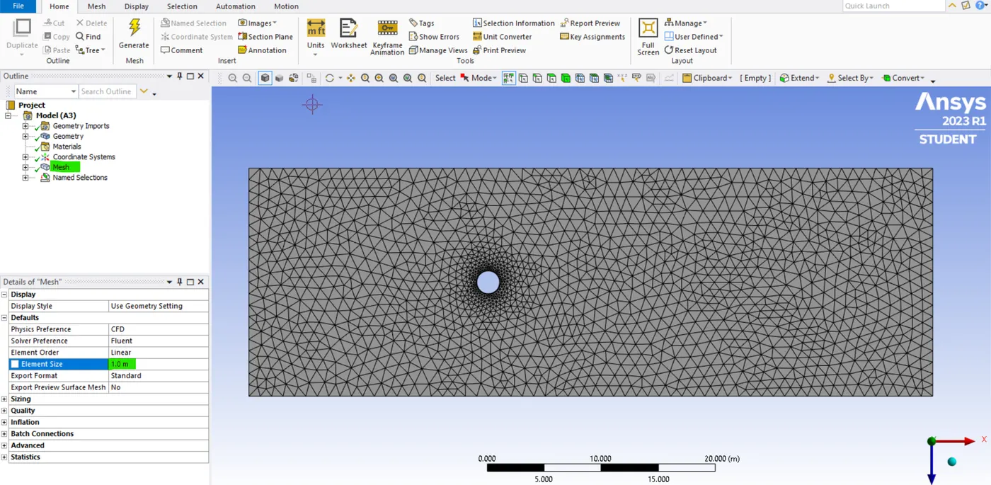
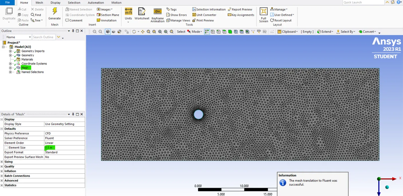
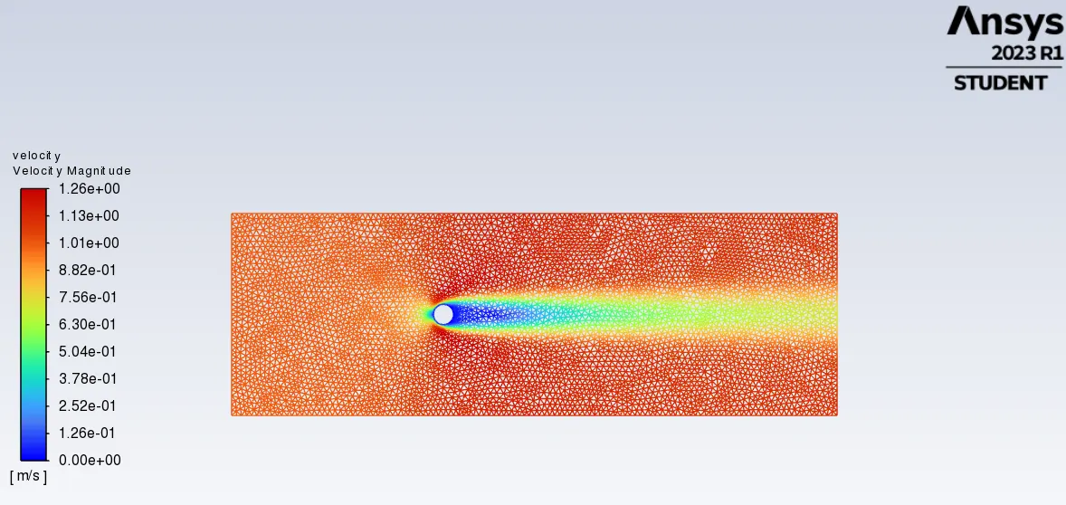
• so, open the mesh block and make sure this time the element size is 0.5 meters. so, close this mesh GUI update this block, and also update the setup as now open the set GUI. so, here the mesh seems to update and re-initialize everything and the no.of.iteration is 350 and hit the calculate.
• so, this time I think I saw a very small blip but it doesn't mean anything. So in my animation, there is no vertex shedding. so, I'm going to refine my mesh one more time.

   

   

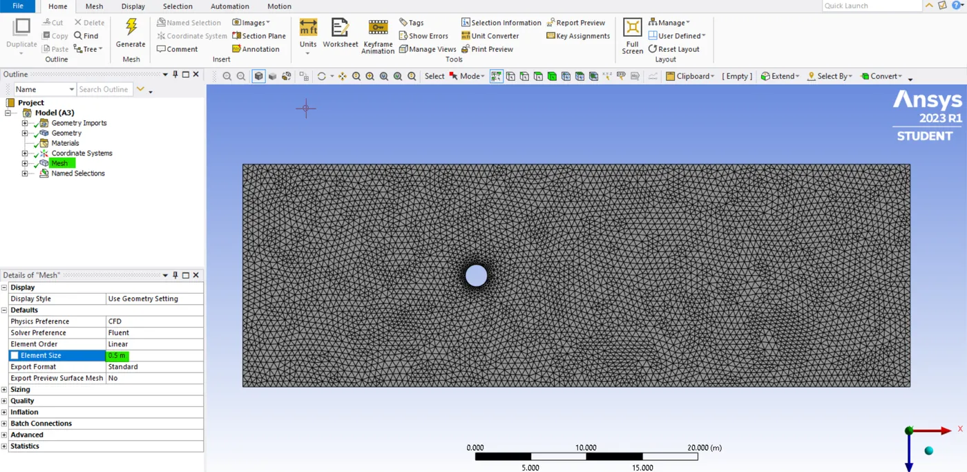
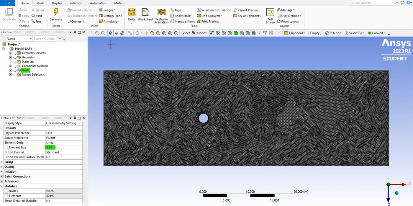
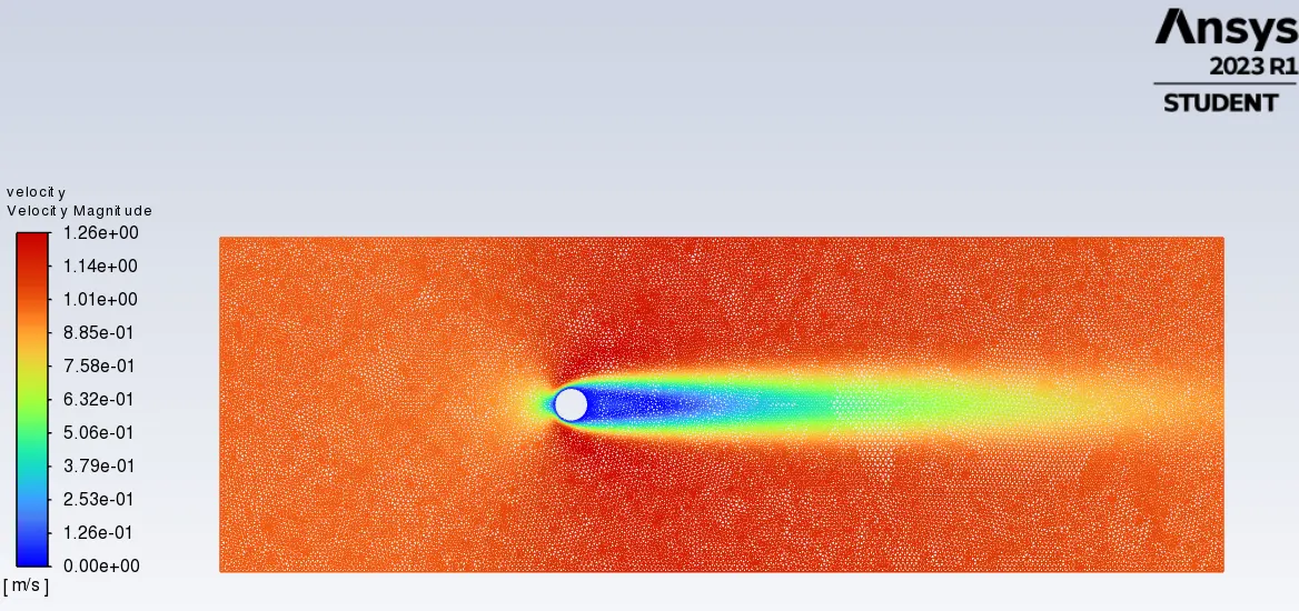
• so, the thing is we need to do this process that we are trying to follow. so, this process is called a consistency check or grid dependency check. so, just close the setup GUI. and let's go to the mesh GUI we need to tune our element size from 0.5 meter to 0.25 meter and our mesh is updated as well.
• Now open the setup GUI and we can see our mesh looks super fine. so, let's re-initialize everything one more time and hit the calculate.

  

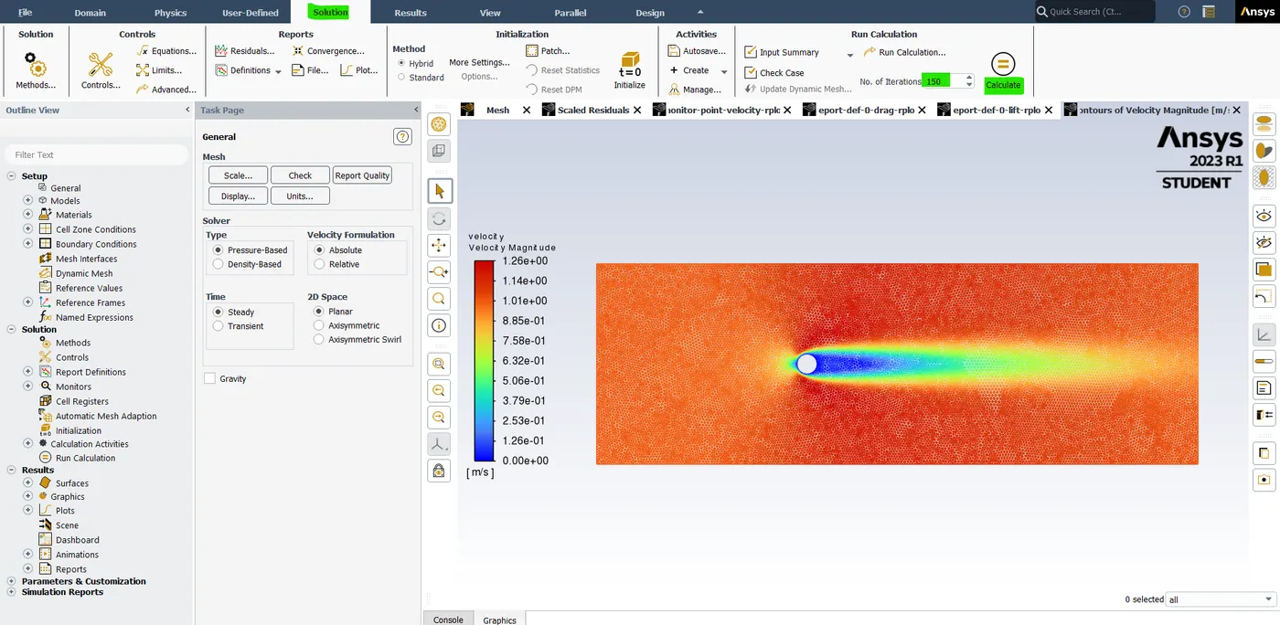
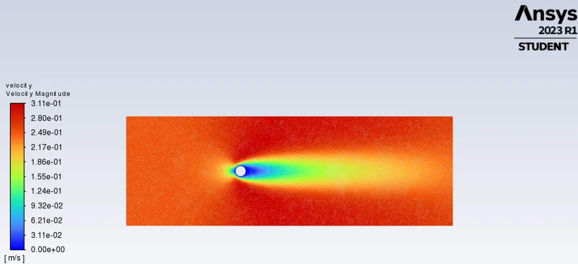
• so, one thing here we need to understand that is when you refine the mesh then we need to simulate for a much longer time. so it doesn't reach the steady state value. we are going to run it for another additional 150 iterations and hit the calculate.
• so, now I'm going to go to the solution playback and play the animation because the information is still not through the outlet. so it means we might have to run this simulation for a longer period. so, when we are making the mesh finer we always need to run it for a longer period.
• so, then run this simulation for 300 more iterations and hit on calculate. Already we have run 500 iterations. now another 300 more.
• so, the calculation is completed and still there is no vertex shading happening. so, the reason is when the Reynolds number is more than 40 then the flow begins to start. Right now the Reynolds number is less than 40. so go to material property -> increase the viscosity slightly then we can capture the vertex shedding.

   

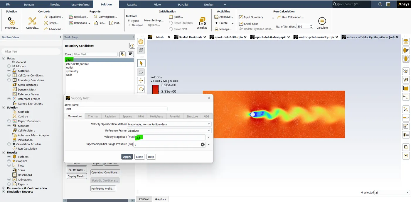
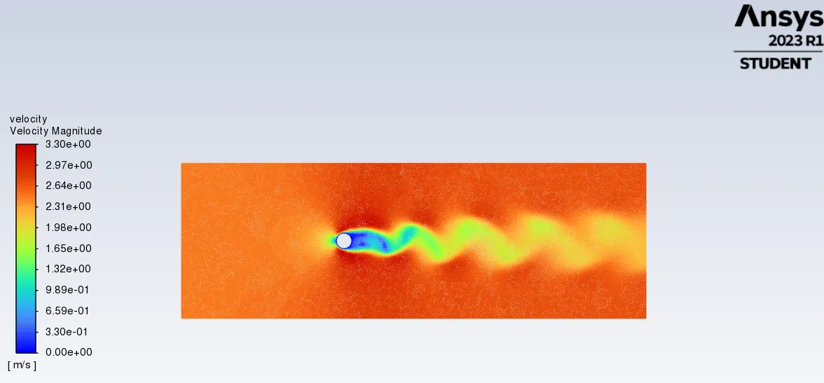
• just change the viscosity from 0.05 to 0.045 click on change save and close the tab. so, now re-initialize everything and enter the no.of.iteration as 350 and hit on calculate.
• so my monitor point velocity is dropping as usual and this is going to start hitting the steady value. so, now just we are going to run another 600 iterations. but it did not help as well. so, what next we are going to do is I'm going to push my Renold number from 0.045 to 0.02 value where I know for sure that there is going to be a lot of vertex shedding and that is our last case which is our last case which is our Renolds number of 100. or we also change to increase the velocity of inlet boundary conditions. 
• so, just go to the material property and change the viscosity to 0.02. so, that's a smaller number, and click change/save. and now re-initializeing everything enter the 350 iteration and hit on calculate.
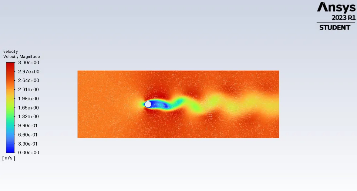
• so, let's look at our other point velocity there it looks like we can see after 160 things are starting to oscillate and if I'm going to see my velocity plot there is a vertex shedding occurred.

     

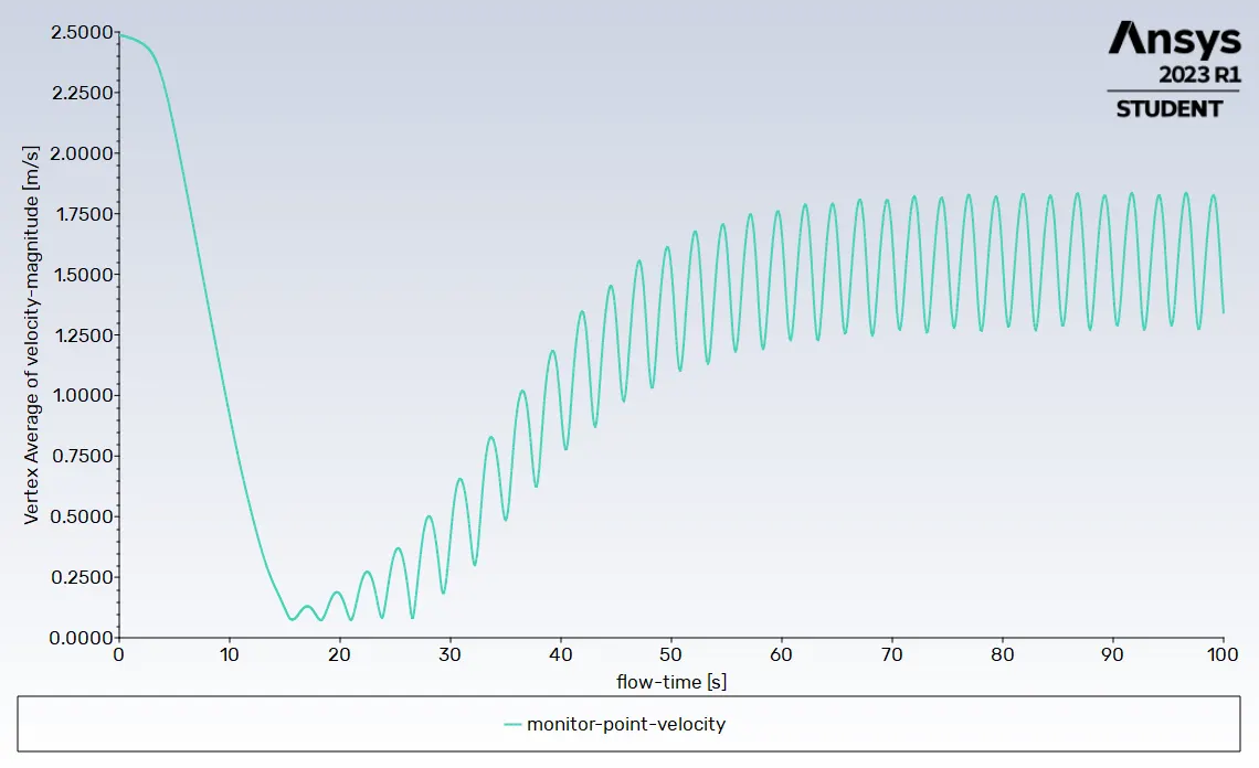
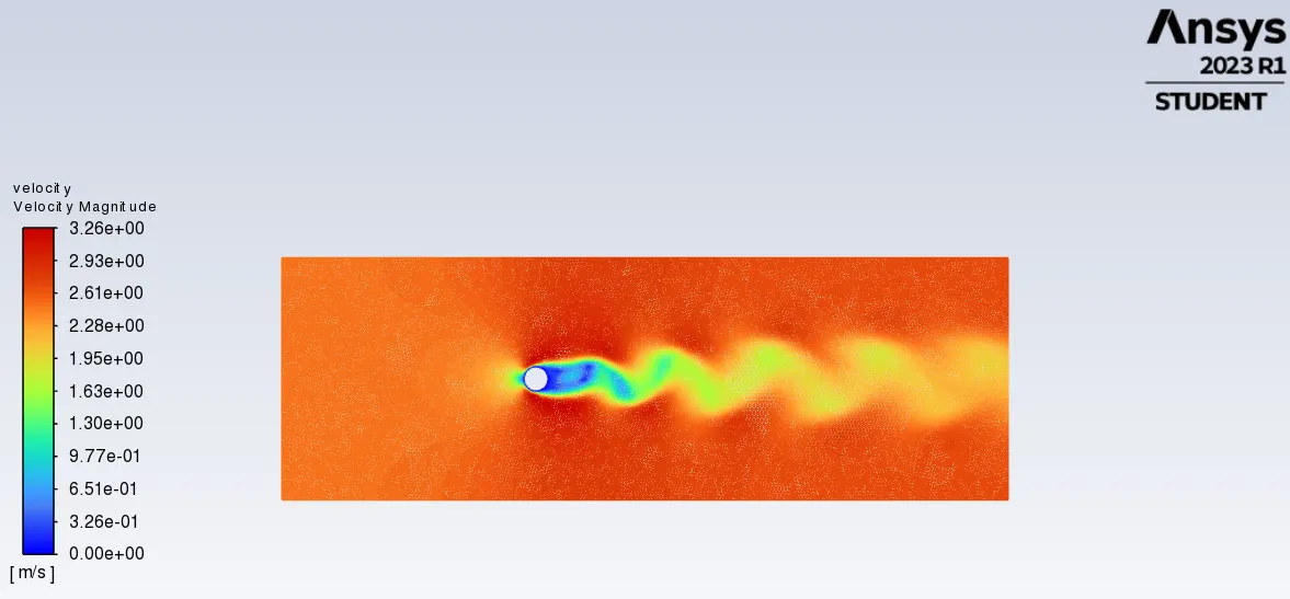
• but if I look at the monitor point you can see the solution has still not reached a steady state value. so, that means we have to run this simulation a bit longer. so, after we ran this simulation, it looked fine, and the vertex shedding also occurred.

• And also you can see that there is a particular frequency to do this oscillation if I measure peak to peak. and if I know the time then I can calculate the actual vertex shedding frequency from which I can calculate the "Strouhal number". And we are using an unsteady-state simulation.
• so, the steady state simulations are typically performed to get your find answers. so, any intermediary solution that you get is not accurate meaning at 250 iterations I got a particular value of velocity.
• so, this does not correlate to a particular time and I think this is why we aren't getting a perfect result.
• anyway we won't be able to calculate the frequency parameter. it means the vertex shedding frequency parameter. In other words, we know how many times a second the velocity flips like this. so, I won't be able to calculate this because there is no time parameter.

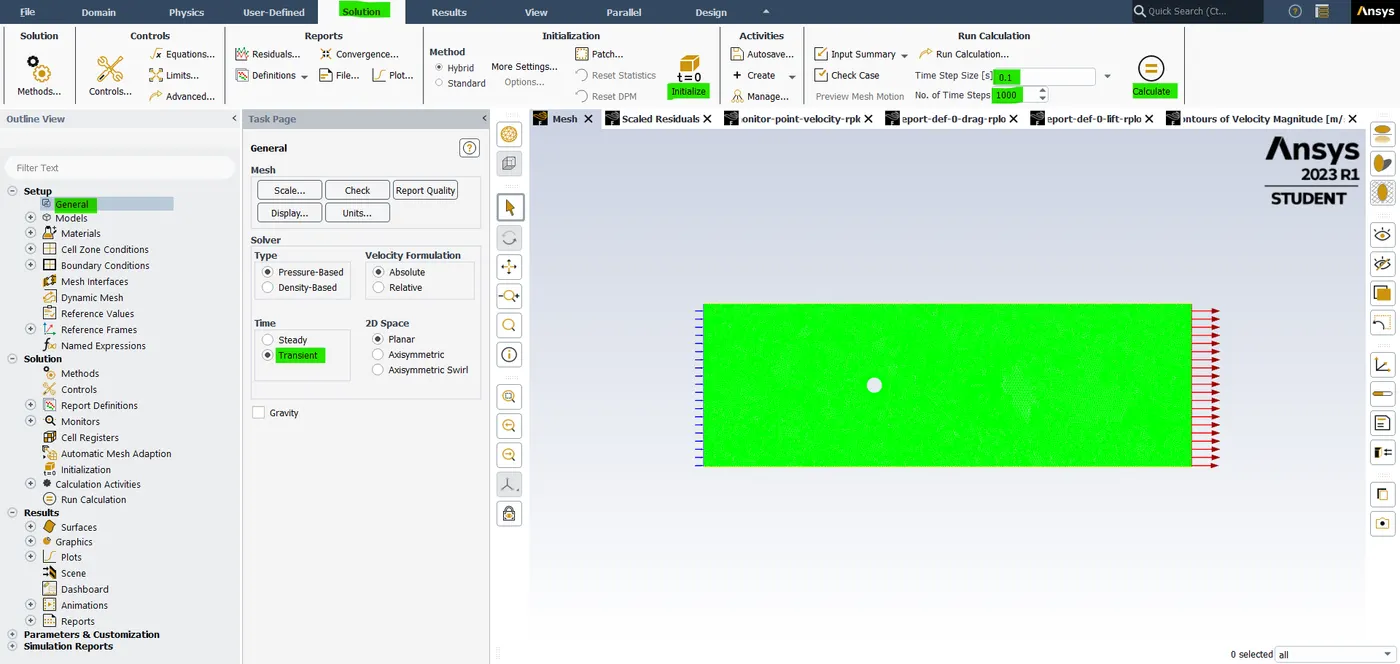
• And that's why we need to run "Transient simulations". so, in this transient simulation what we do is we solve the equation accurately meaning that we can trust the result.
• And I think my guess is because of that we are unable to see the vertex shedding exactly at Renolds number 40. so, we are going to set up solver -> change to "Transient simulation".
• so now go to solving enter the time step size 0.1 sec and enter the on. of the time step is 500. and got our material property and changed my viscosity to 0.05 which is an original value that we added so, re-initialize everything and I'm going to run this simulation from the first.
• so, it took a lot of time to solve but it did solve and the exerting thing is we were able to see the cortex shedding, whereas when we did the steady-state simulation. we were not able to see it. then the problem is transient. In other words when we are looking for a quantity that's changing as a function of time you better use a transient simulation. and on top of that, our mesh needs to be refunded for a finer size.

3. Post-processing (Result):-

RESULT:-

plots:

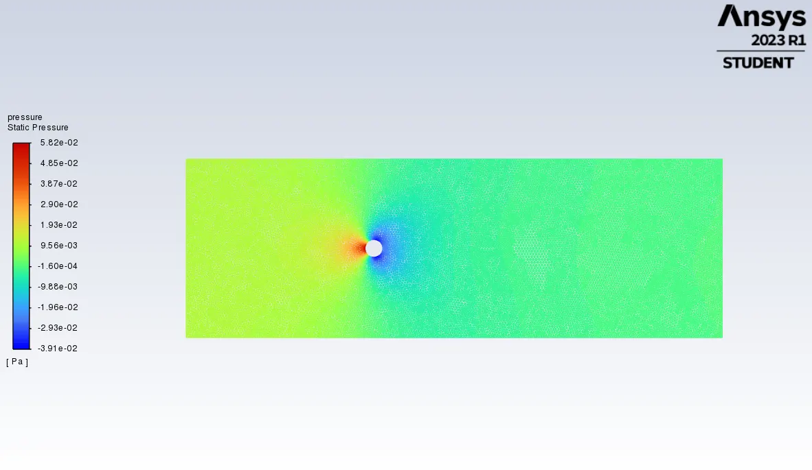
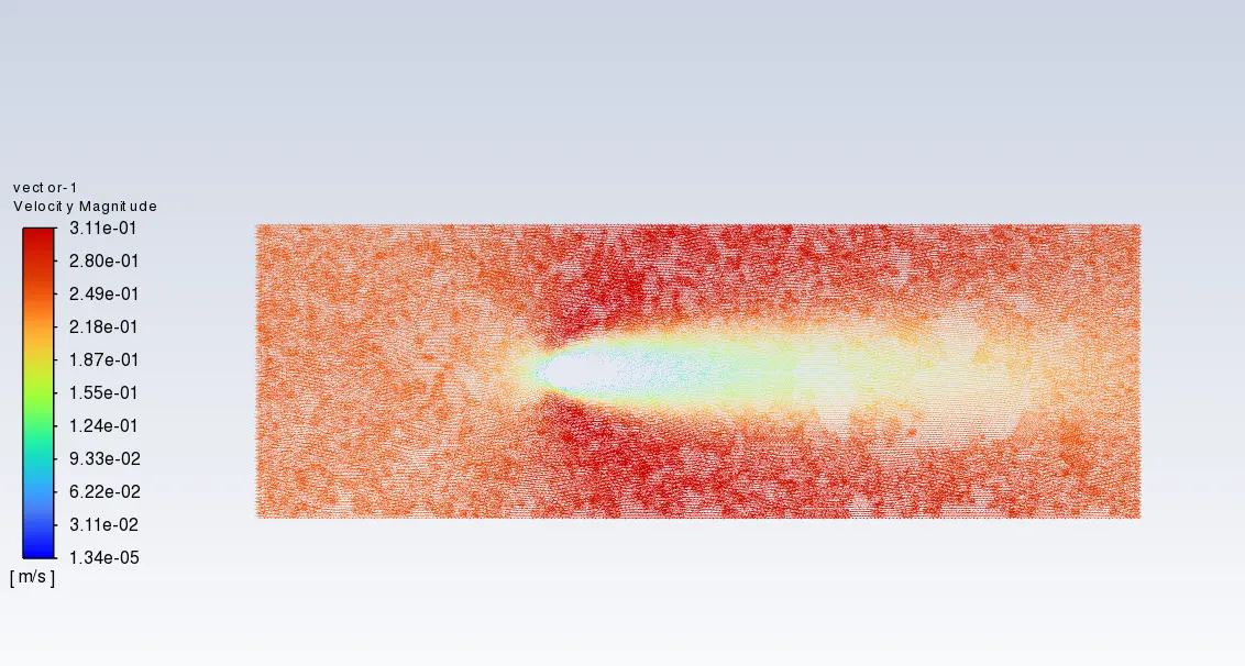
• Case-1: Re-10, inlet velocity=0.25, steady-state solver.

Scaled Residual:

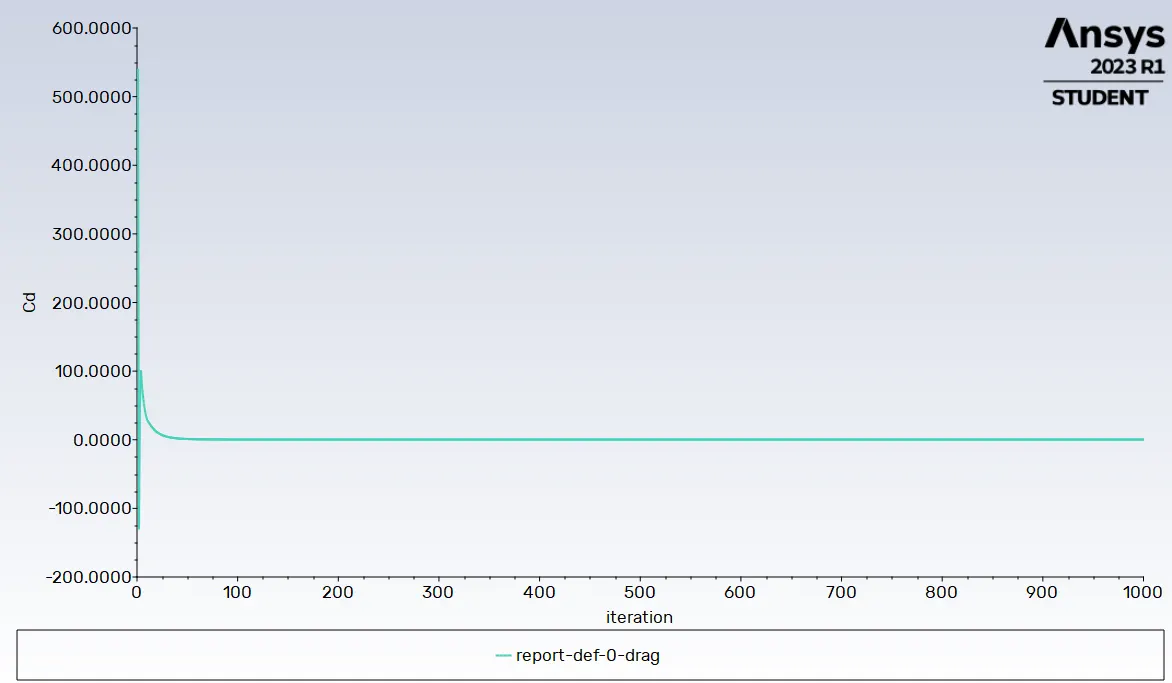
Drag plot:

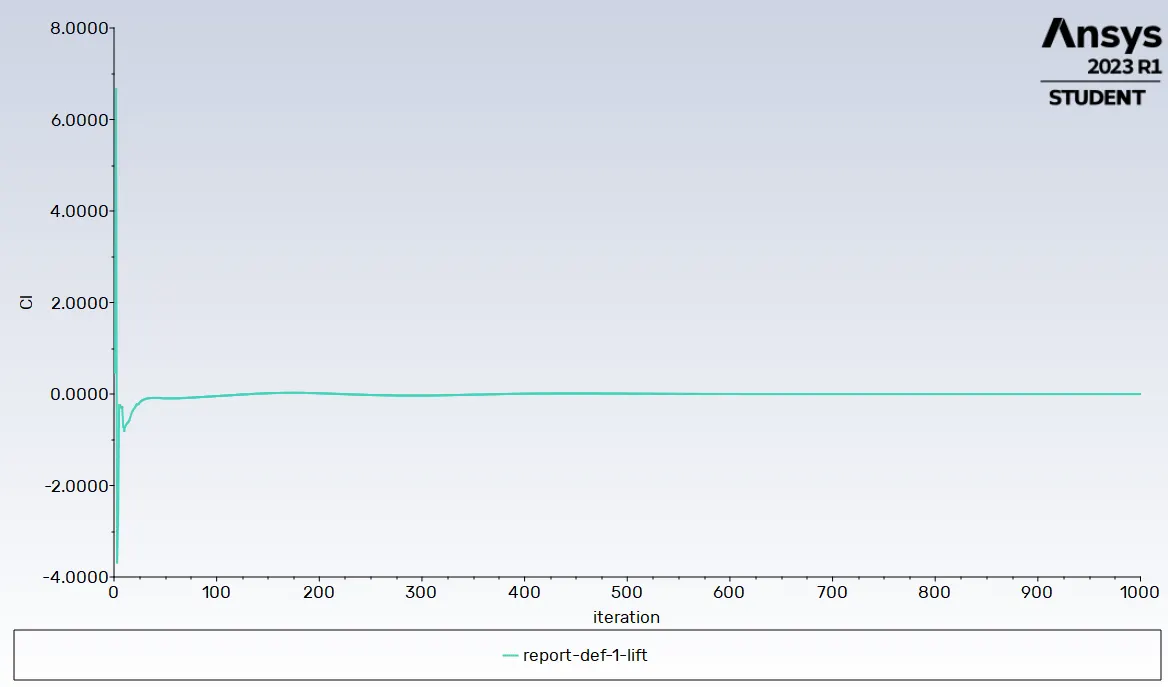
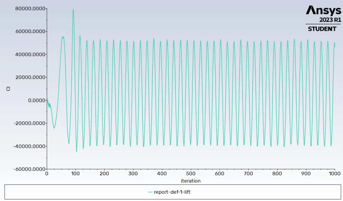
Lift plot:

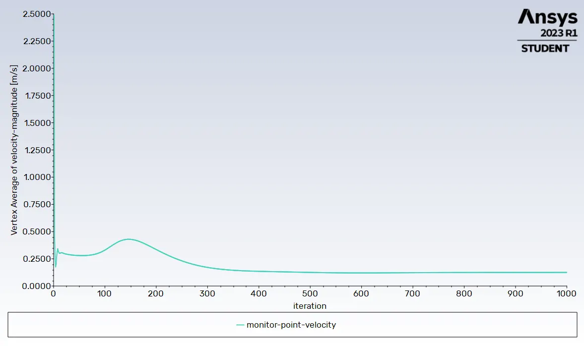
Vertex average velocity plot:

Velocity contour:

Pressure contour:

Vector velocity contour:

 

plots:

• Case-2: Re-100, inlet velocity=2.5, steady-state solver.

Scaled Residual: 

  

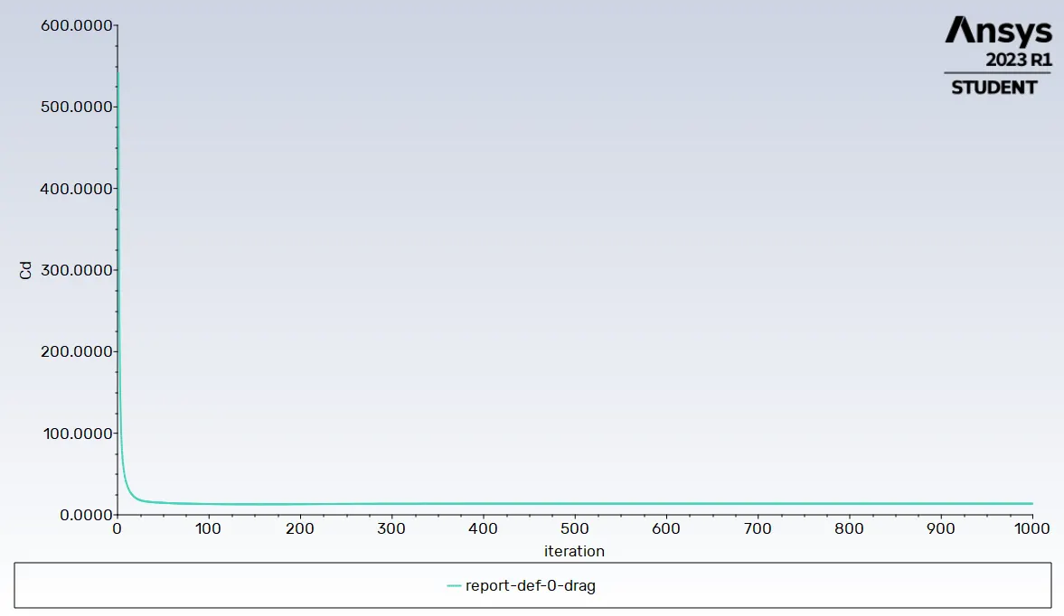
Drag plot:

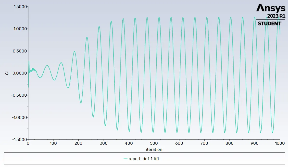
Lift plot:

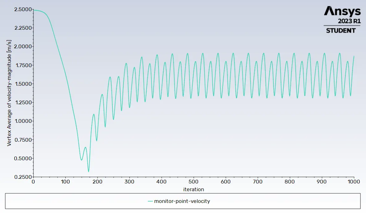
Vertex average velocity plot:

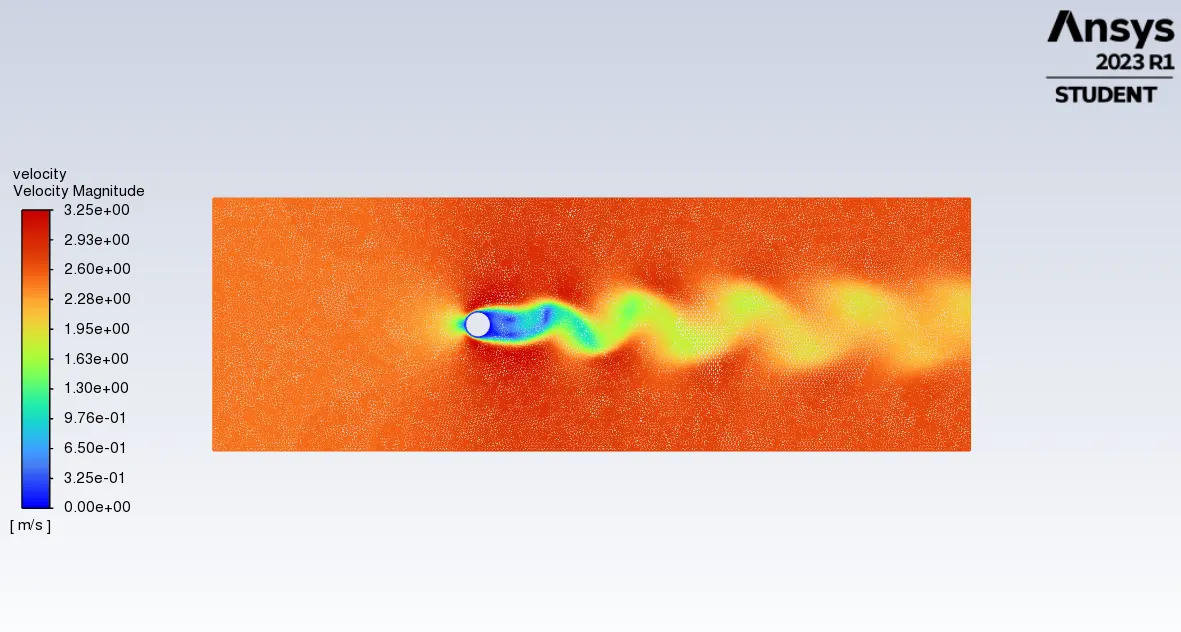
Velocity contour:

Pressure contour:

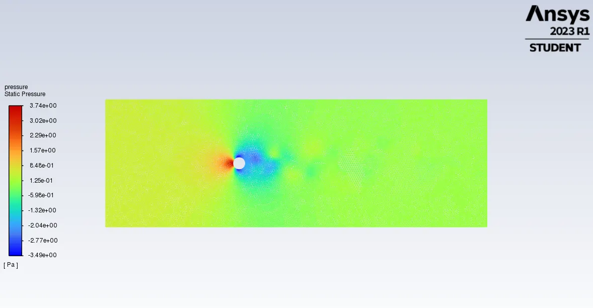
Vector velocity contour:

 

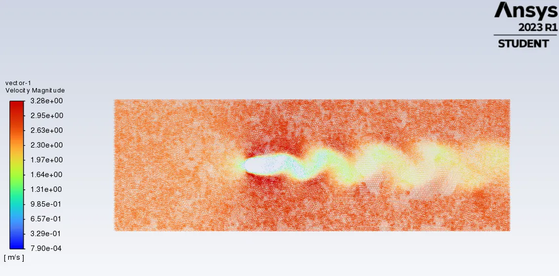
• Case-3: Re-100, inlet velocity=2.5, unsteady-state solver.

Scaled Residual:

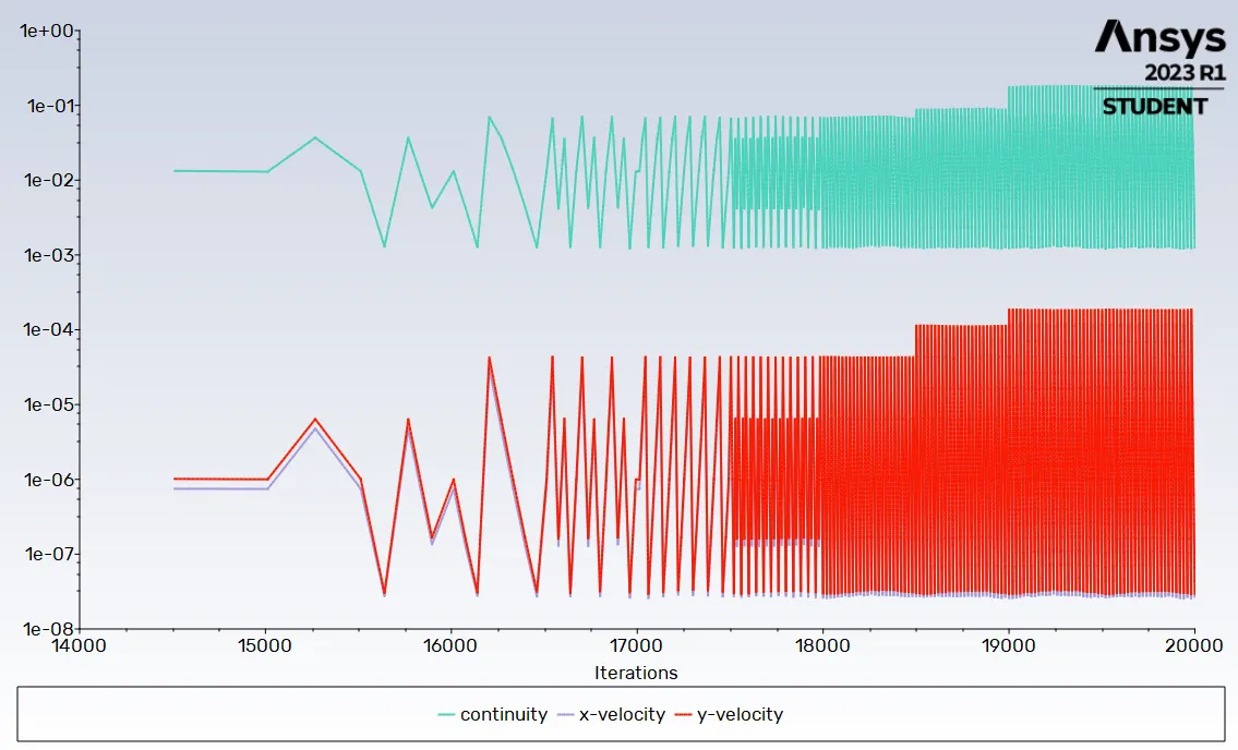
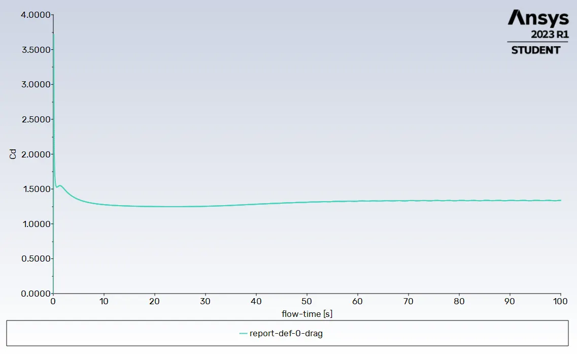
Drag plot:

Lift plot:

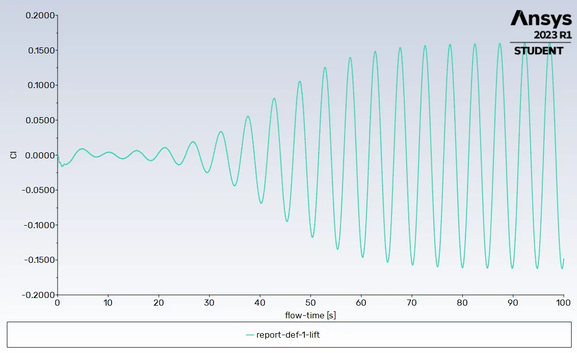
Vertex average velocity plot:

Velocity contour:

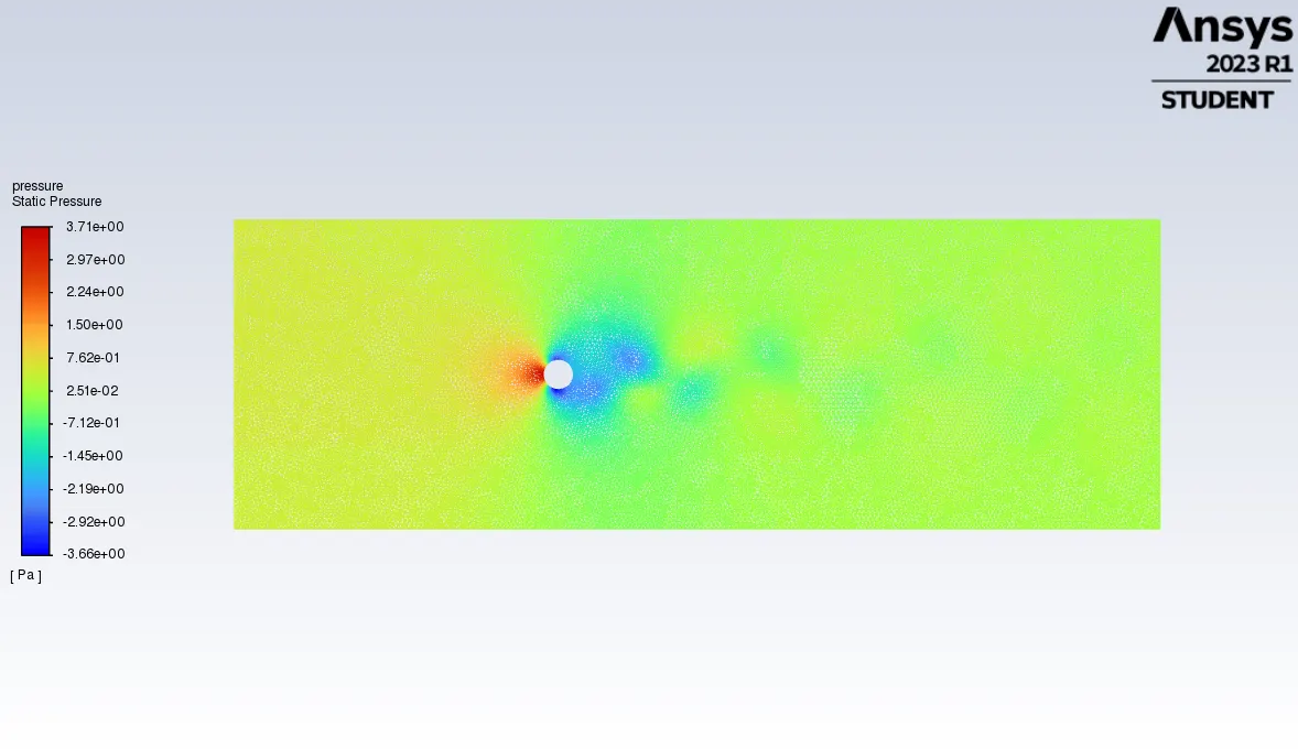
Pressure contour:

Vector velocity contour:

 

plots:

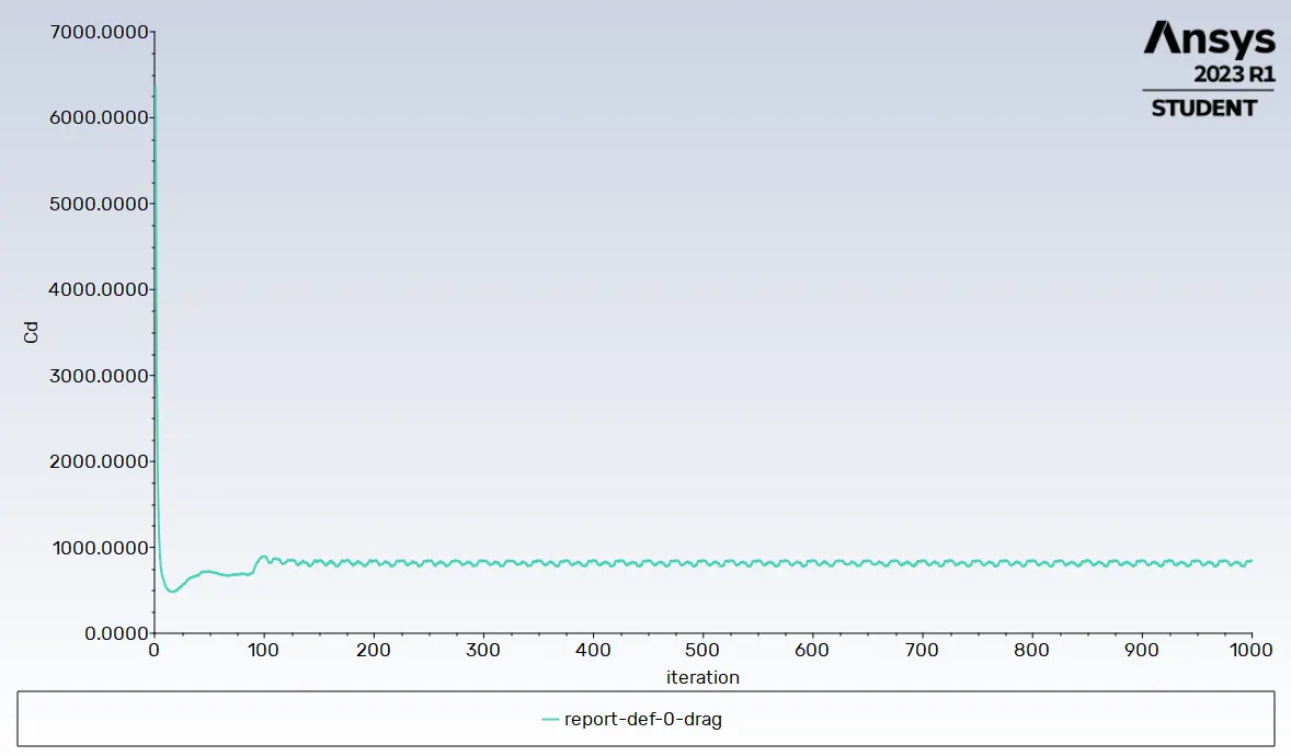
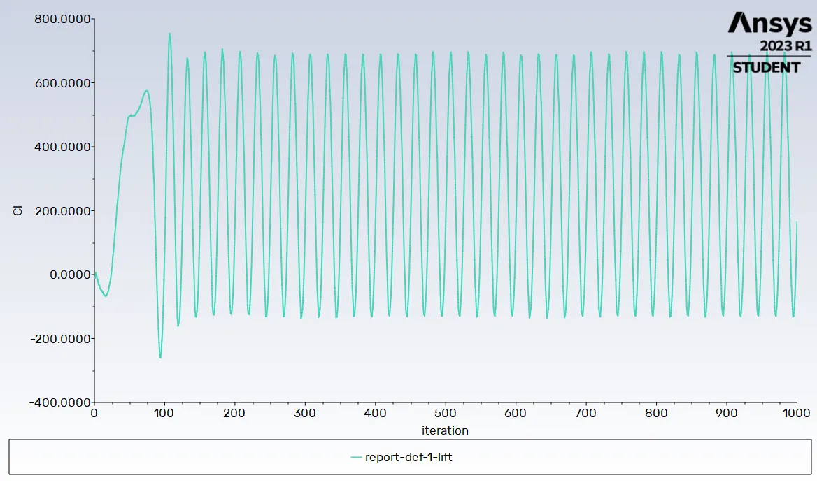
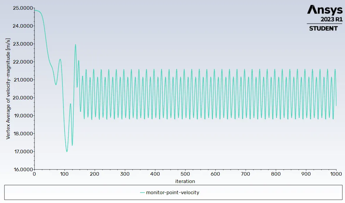
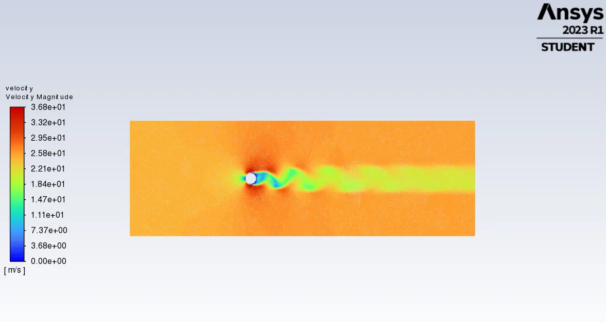
• Case-4: Re-1000, inlet velocity=25, steady-state solver.

Scaled Residual:

Drag plot:

Lift plot:

Vertex average velocity plot:

Velocity contour:

Pressure contour:

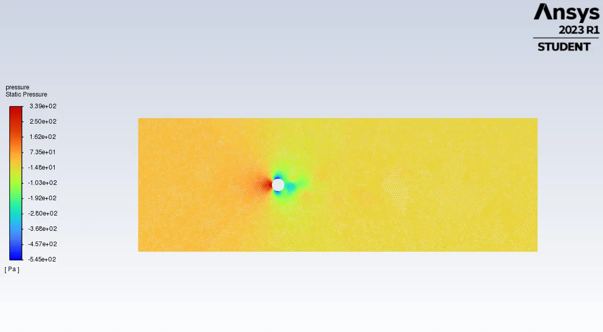
Vector velocity contour:

 

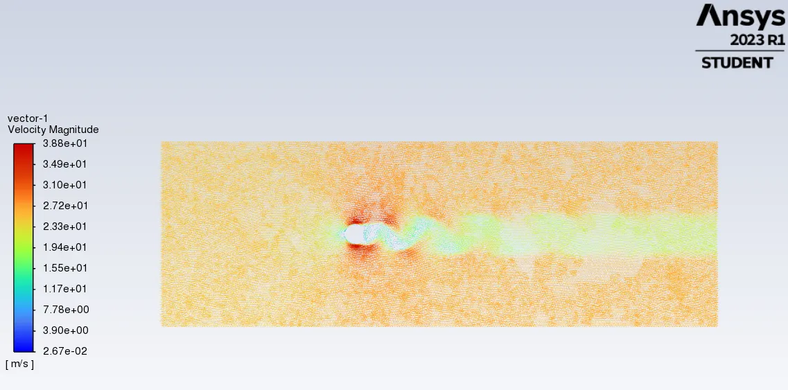
ANIMATION VIDEO:-

https://drive.google.com/drive/u/1/folders/1k1cH-iGC2-STt6QKdQUY_B89QRwmjBmP 

plots:

• Case-5: Re-10000, inlet velocity=250, steady-state solver.

Scaled Residual:

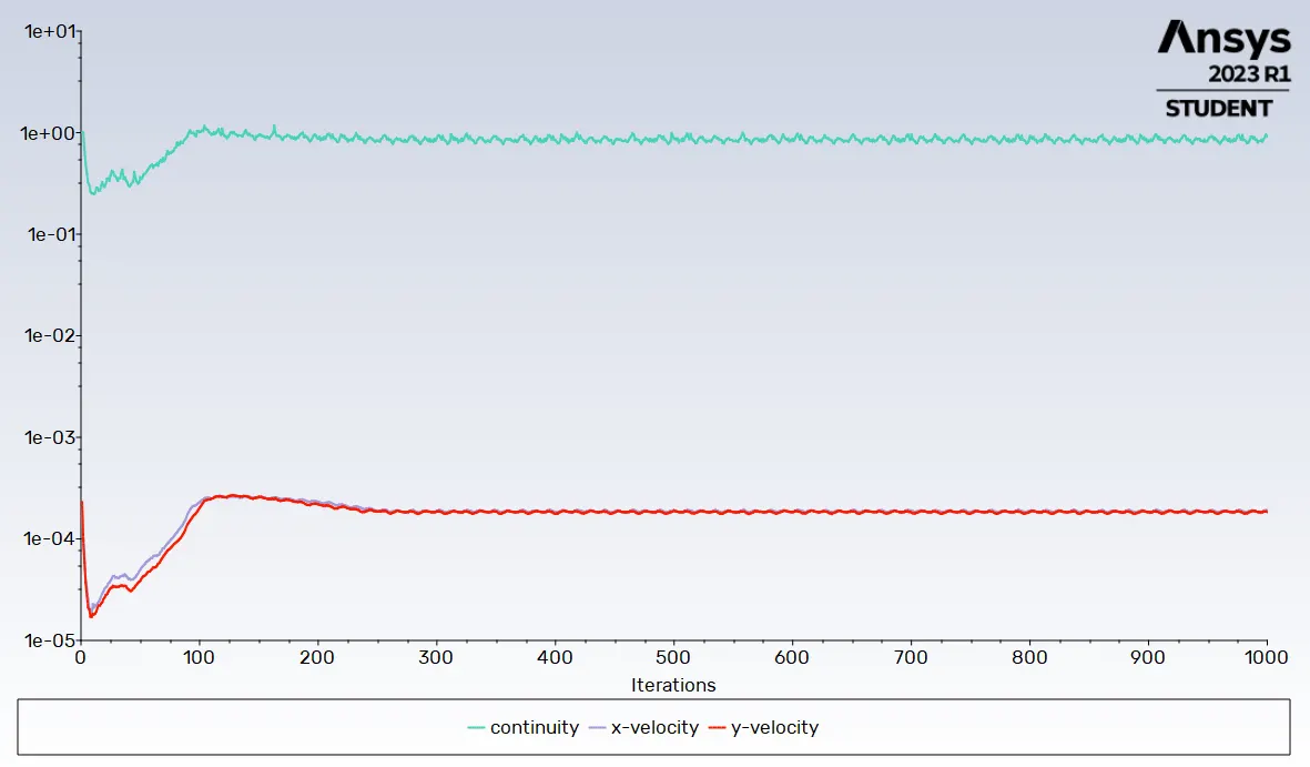
Drag plot:

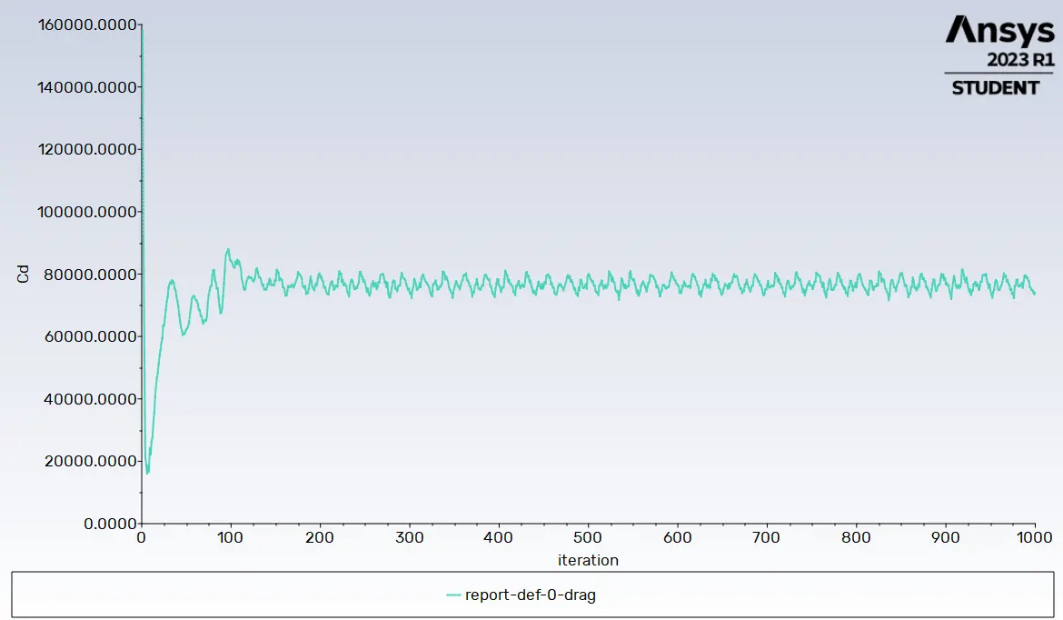
Lift plot:

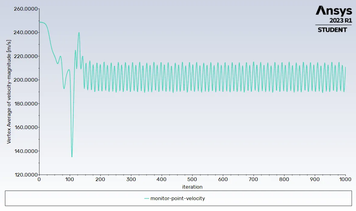
Vertex average velocity plot:

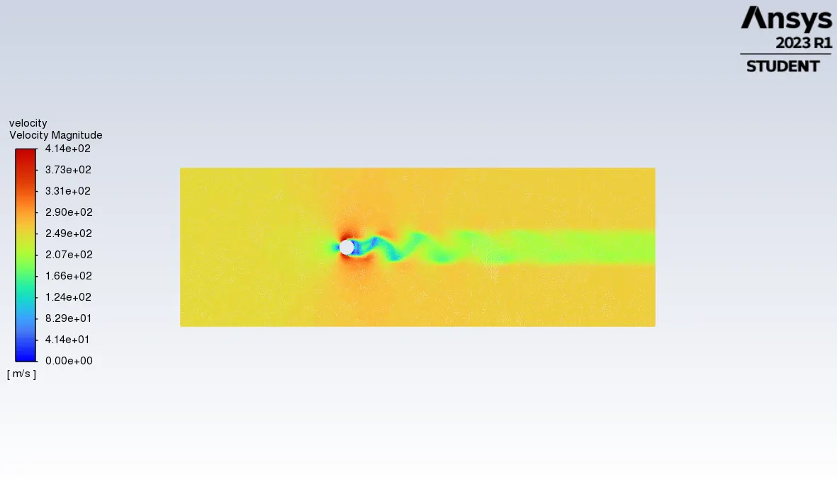
Velocity contour:

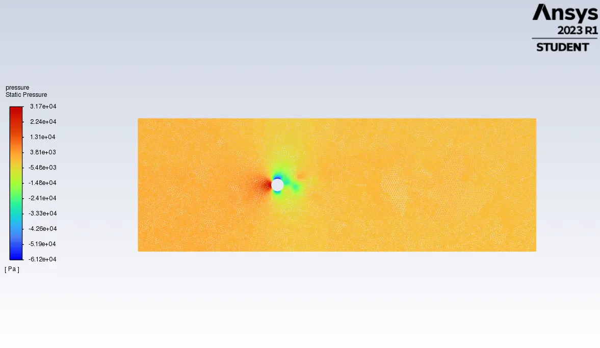
Pressure contour:

Vector velocity contour:

 

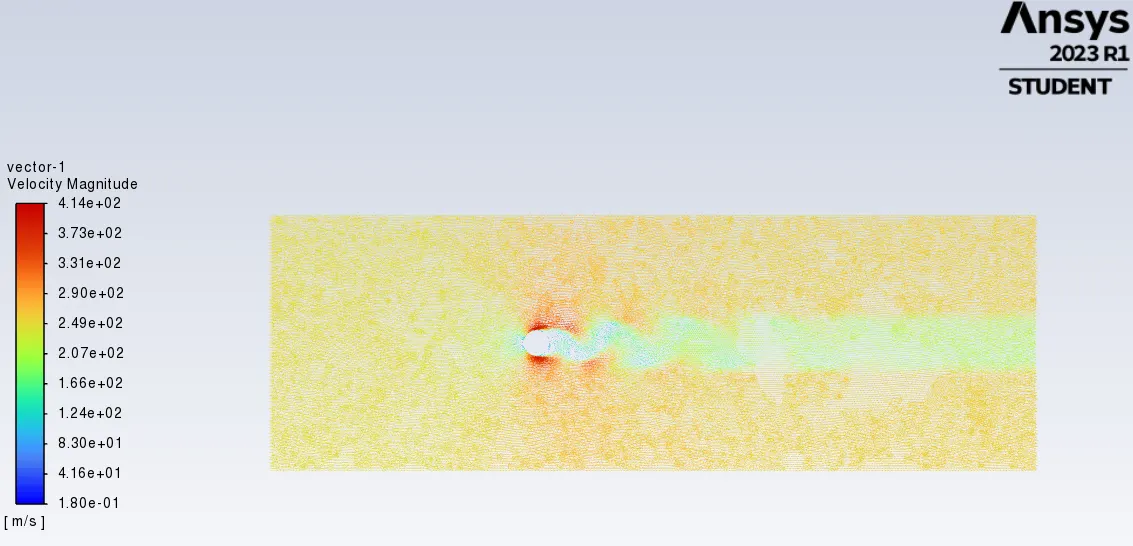
plots:

• Case-6: Re-100000, inlet velocity=2500, steady-state solver.

Scaled Residual:

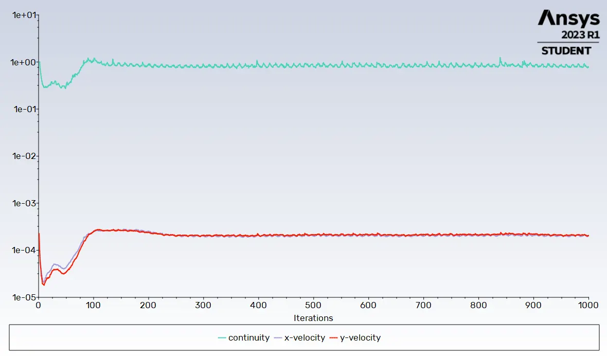
Drag plot:

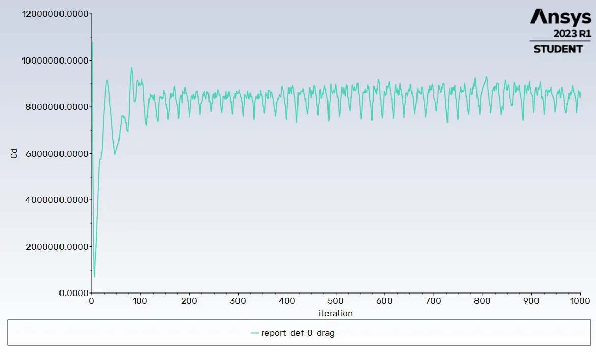
Lift plot:

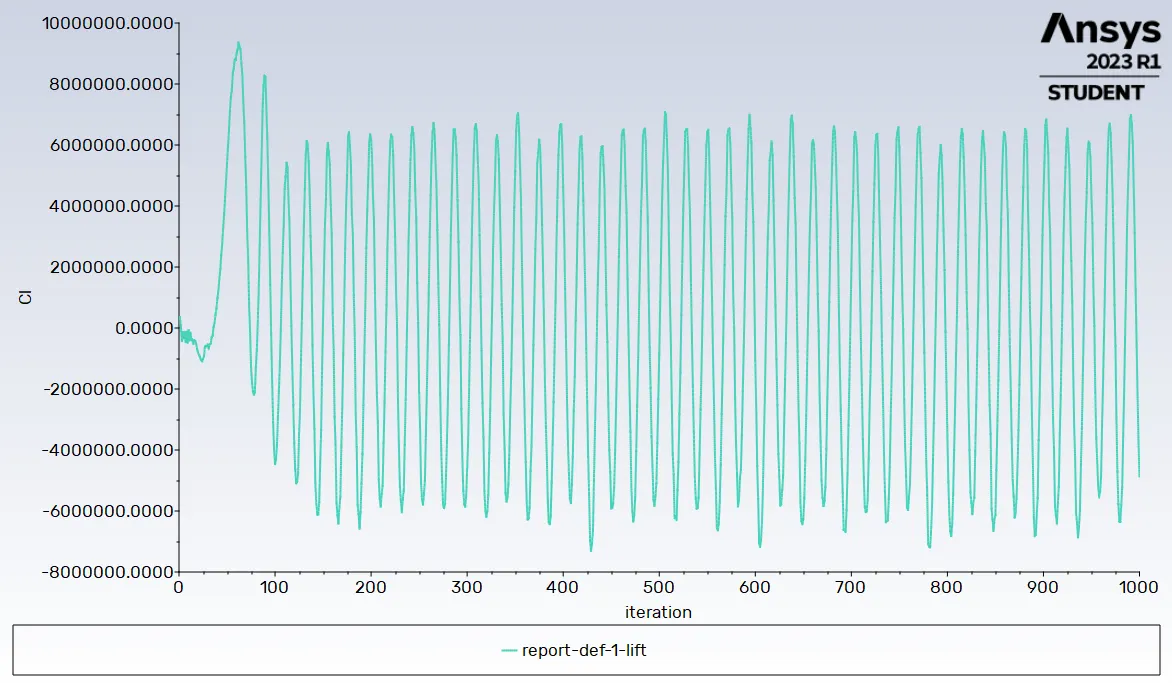
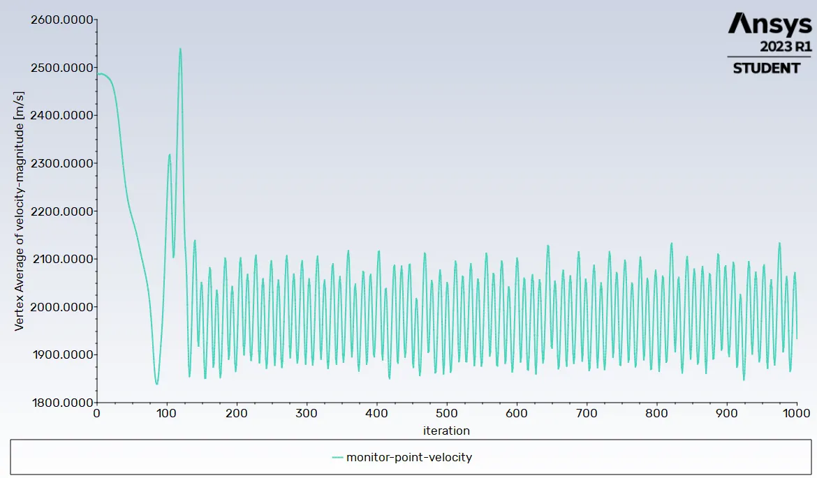
Vertex average velocity plot:

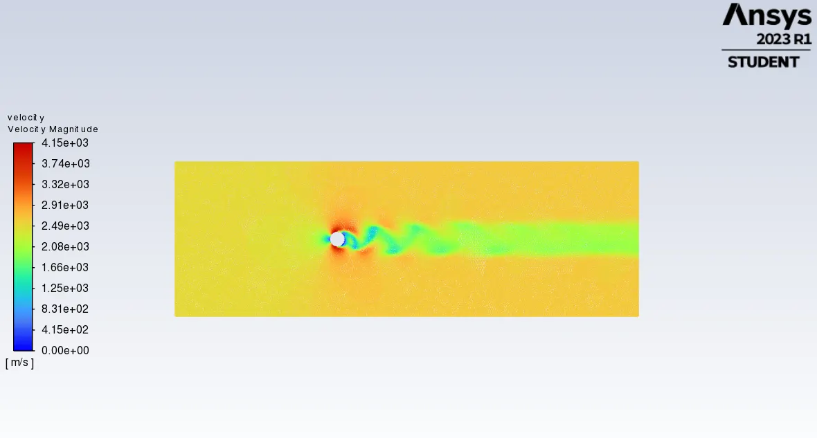
Velocity contour:

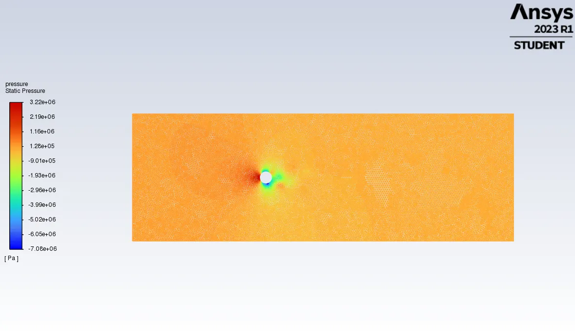
Pressure contour:

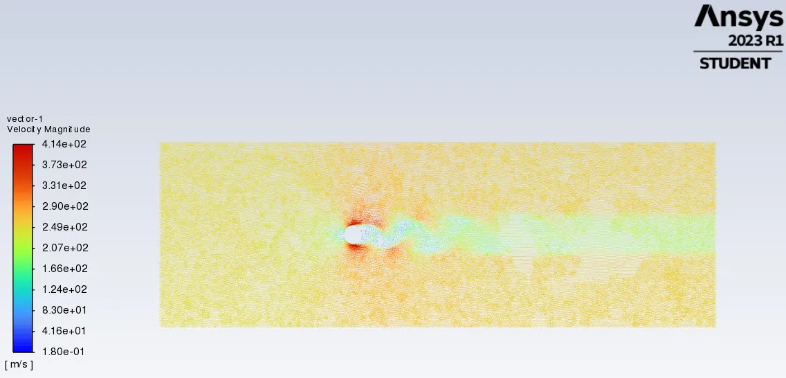
Vector velocity contour:

 

CONCLUSION:-

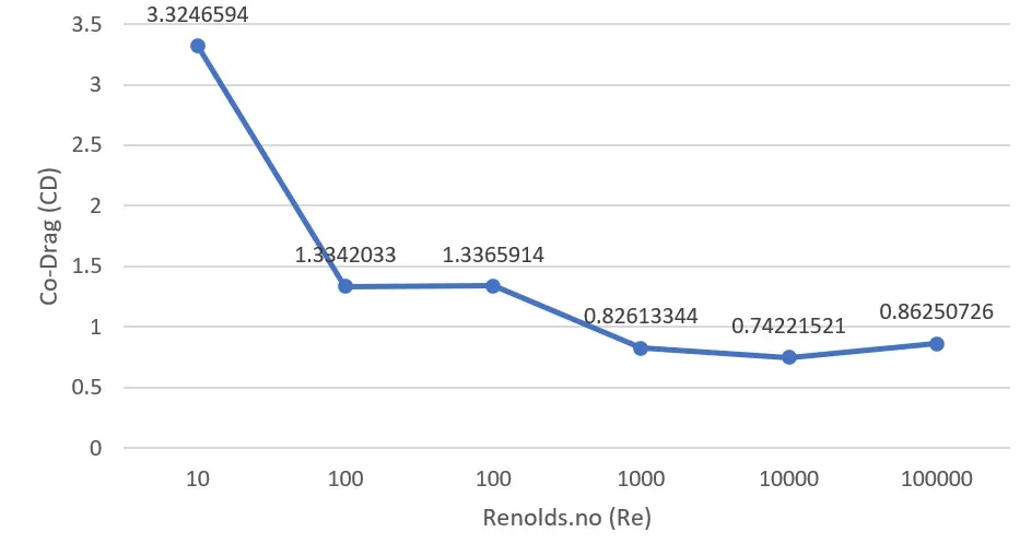
• The Following table shows the value of the coefficient of drag (C_d) and coefficient of lift (C_l) for the certain Reynolds no. and the velocity.
• Mean Vertex average formula is min value - max value / 2. so when the flow reaches a convergence criterion or steady state. so, we need to measure the peek-to-peek value in the monitor point velocity graph. and then divide that value by 2. so, we will get the mean vertex average value.

Cases	Type of flow	Reynolds NO. (Re)	Velocity (m/s)	Coefficient of Drag(Cd)	Coefficient of Lift(Cl)	Mean Vertex avg.
1.	steady-state flow	10	0.25	3.3246594	-0.0033857384	0.1248
2.	steady-state flow	100	2.5	1.3342033	0.10414476	0.29865
3.	unsteady-state flow	100	2.5	1.3365914	-0.14834956	-0.71034
4.	steady-state flow	1000	25	0.82613344	0.16287877	-1.38025
5.	steady-state flow	10000	250	0.74221521	-0.38565073	-11.7124
6.	steady-state flow	100000	2500	0.86250726	-0.34611277	-124.82295

• The following graph shows the drag plots and the Reynolds no. plots for each case. And here when my Reynold no. increases then the coefficient of drag is decreased. This happens because the flow separation starts after a certain value of the Reynolds number and the coefficient of drag is decreased. 
• The drag is inversely proportional to the fluid flow. In every case, the fluctuations happened concerning the Reynold no. and velocity so it indicates the vortex shedding has occurred. except for case 1, there is no vortex shedding due to the small Renolds no. and velocity.
• The monitor point is used to monitor the velocity and pressure with the help of sensors and we can also monitor the flow whether the flow has converged or not. the mean velocity average is what we can not use to analyze the result. 
• The animation video was created for case 4 and the vertex shadings are formed behind the cylinder wall.