Week 2 - Flow over a Cylinder.
AIM:
- To simulate the flow over the cylinder for steady state and unsteady state condition. Check this simulation for the Reynolds number of 100 and make the plot of generated data and check for the vortex shedding.
- To find out the strouhal number for the given reynolds number of 100.
- To calculate drag & lift coefficient for the flow over a cylinder for the series of Reynolds Number of 10, 100, 1000, 10000, & 100000 under steady state condition
DEFINITION:
Vortex Shedding:
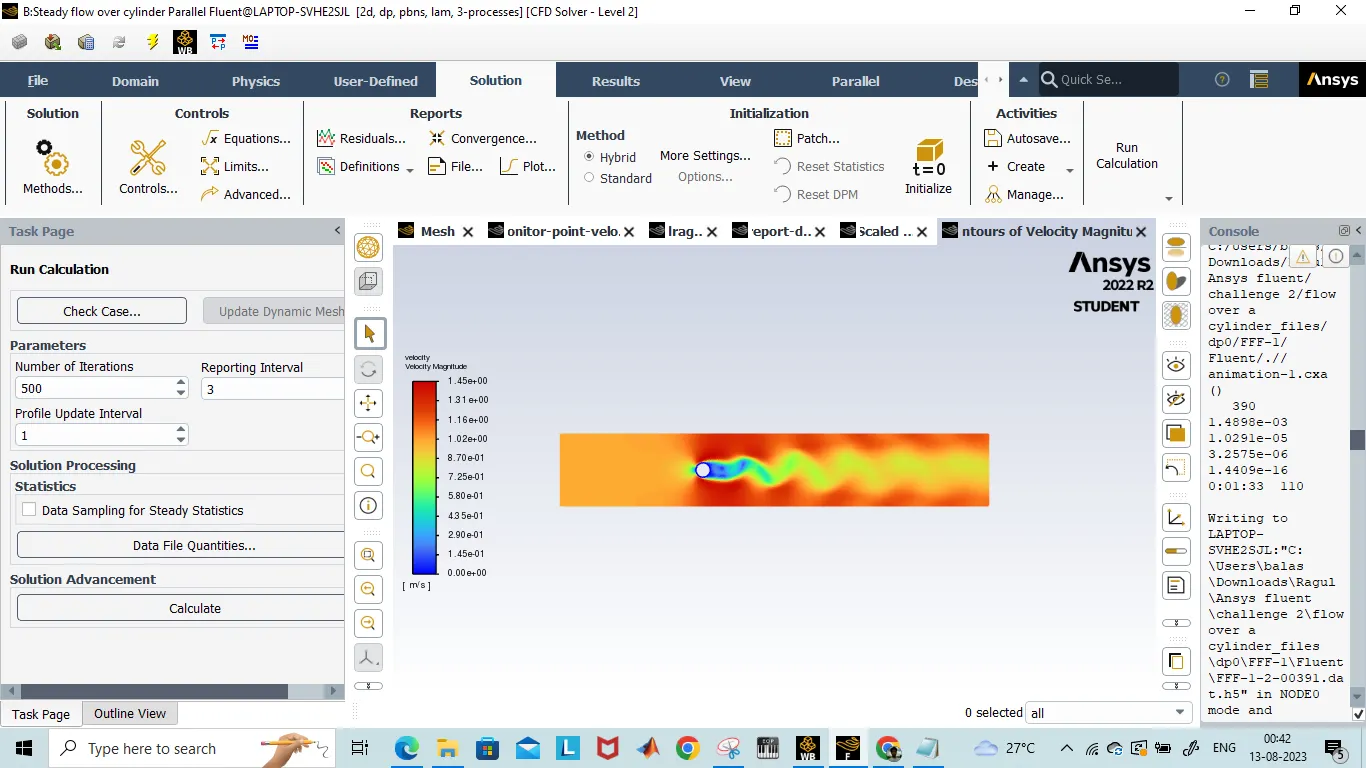
It is a phenomenon that when the flow crosses the bluff body, vortices are shed alternately from one side to the other, & where alternating low-pressure zones are generated to the downside of the bluff body giving rise to a fluctuating force acting at right angles to the flow direction. A vortex shedding forms only at a certain range of flow velocities, specified by a range of Reynolds numbers (Re), typically above a limiting Re value of about 90.
Karman vortex street:
In fluid dynamics, a Karman vortex street (or a von Karman vortex street) is a repeating pattern of swirling vortices, caused by a process known as vortex shedding, which is responsible for the unsteady separation of flow of a fluid around blunt bodies.
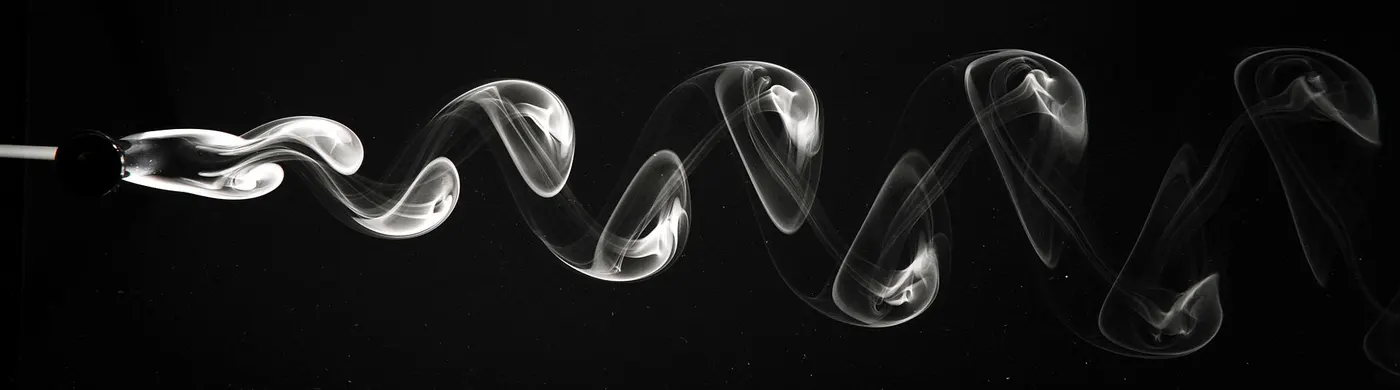
Reynolds number:
The Reynolds number is the ratio of inertial forces to viscous forces. The Reynolds number is a dimensionless number used to categorize the fluids systems in which the effect of viscosity is important in controlling the velocities or the flow pattern of a fluid. Mathematically, the Reynolds number, NRe, is defined as

- ρ is the density of the fluid (kg/m3)
- u is the flow speed (m/s)
- L is a characteristic linear dimension (m)
- μ is the dynamic viscosity of the fluid (Pa·s or N·s/m2 or kg/(m·s))
- ν is the kinematic viscosity of the fluid (m2/s).
The Reynolds number is used to determine whether a fluid is in laminar or turbulent flow.
- If Re < 2000>
- If Re > 4000, the flow is called turbulent
- If 2000 < Re>
Strouhal Number:
The Strouhal number represents the ratio of inertial forces due to the local acceleration of the flow to the inertial forces due to the convective acceleration. Depending on the time scale of the problem, this ratio may be of order unity, and therefore its importance is not obvious.
In flows characterized by a periodic motion, the Strouhal number is associated with the oscillations of the flow due to the inertial forces relative to the changes in velocity due to the convective acceleration of the flow field. Thus, an alternative definition of the Strouhal number better suited to periodic flows is given by the following expression

where f is the frequency of vortex shedding, L is the characteristic length (for example, hydraulic diameter or the airfoil thickness) and U is the flow velocity.
- For large Strouhal numbers (order of 1), viscosity dominates fluid flow, resulting in a collective oscillating movement of the fluid "plug".
- For low Strouhal numbers (order of 10−4 and below), the high-speed, quasi-steady-state portion of the movement dominates the oscillation.
- Oscillation at intermediate Strouhal numbers is characterized by the buildup and rapidly subsequent shedding of vortices.
S = 0.20*(1-(20/Re))
S=0.20*(1-(20/100)=0.16
Design Inputs:
Material: Air
Density: 1 kg/m^3
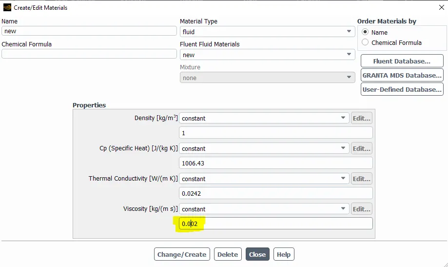
Viscosity: 0.02 NS/m^2
DRAG FORCE:
The resistance force of fluid is known as drag force; this force always acts opposite to the motion of an object which is moving submerged in a certain fluid. Therefore, drag force can also be defined as the force that counterattacks or resists the motion of a body in a fluid. The fundamental nature of drag force is to act in the opposite direction of the flow velocity.
Air resistance can be considered as an example of the drag force because it always resists the terminal speed of an object falling from a certain height.
DRAG COEFFICIENT
When an object moves through a fluid, then to compute its resistance, the coefficient used is known as the Drag coefficient, denoted by Cd. The coefficient of drag is dimensionless, which is helpful in calculating aerodynamic drag and the impact of shape, inclination and conditions of flow in aerodynamics.
Basically, unsharpened and bulky objects will have a high drag coefficient, and streamlined objects will have a lower drag coefficient.
LIFT COEFFICIENT
In fluid dynamics, the lift coefficient (CL) is a dimensionless quantity that relates the lift generated by a lifting body to the fluid density around the body, the fluid velocity and an associated reference area.
CASE – 1: Simulation over the cylinder with a steady and unsteady solver for Reynolds number 100.
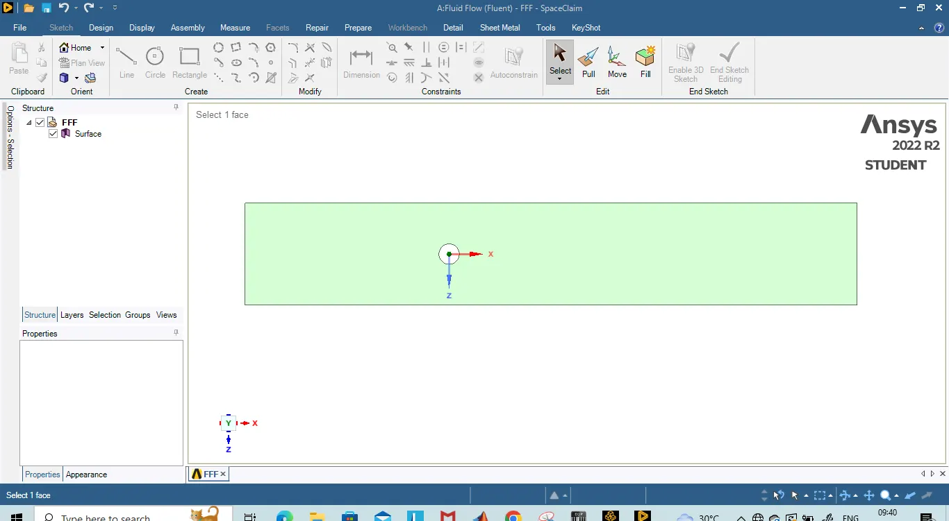
1)Geomentry creation
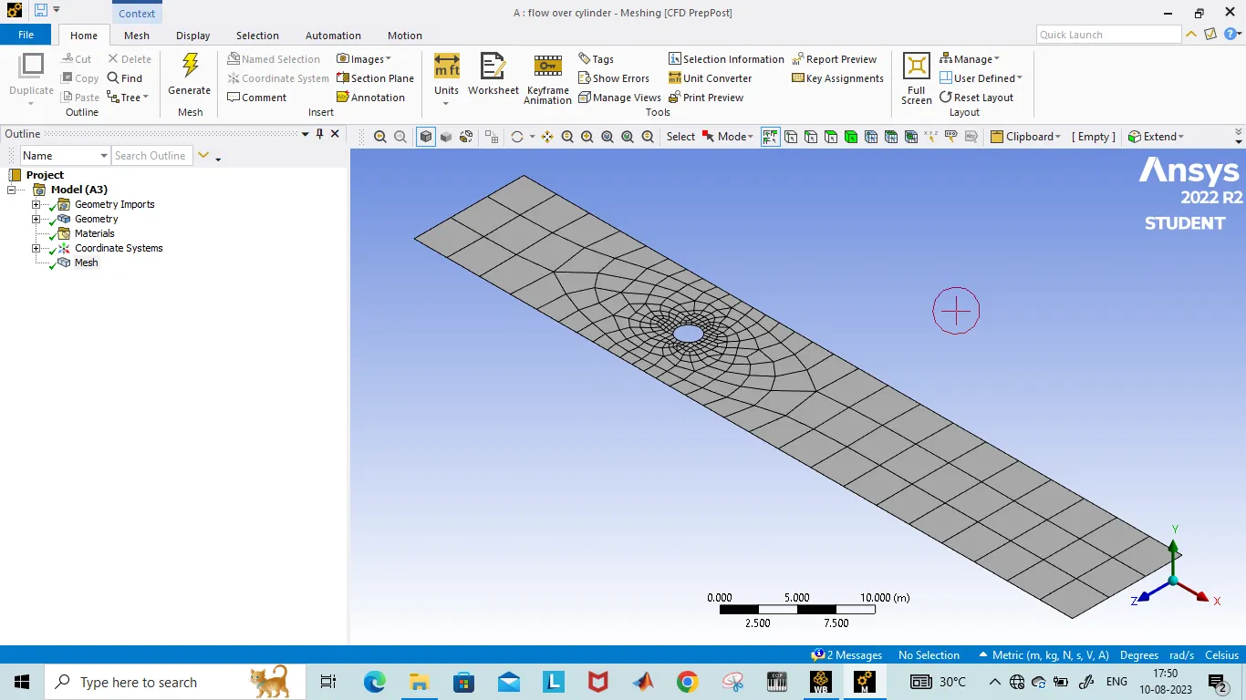
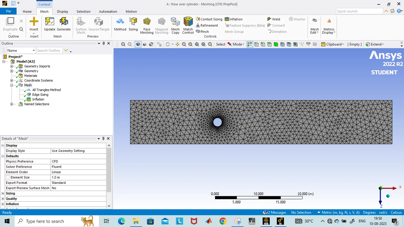
2)Automatic mesh creation by ansys fluent
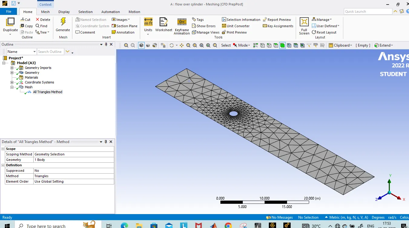
3)Mesh element type is changed to triangles
4)Cylinder 2D view looks like polygon in mesh generation
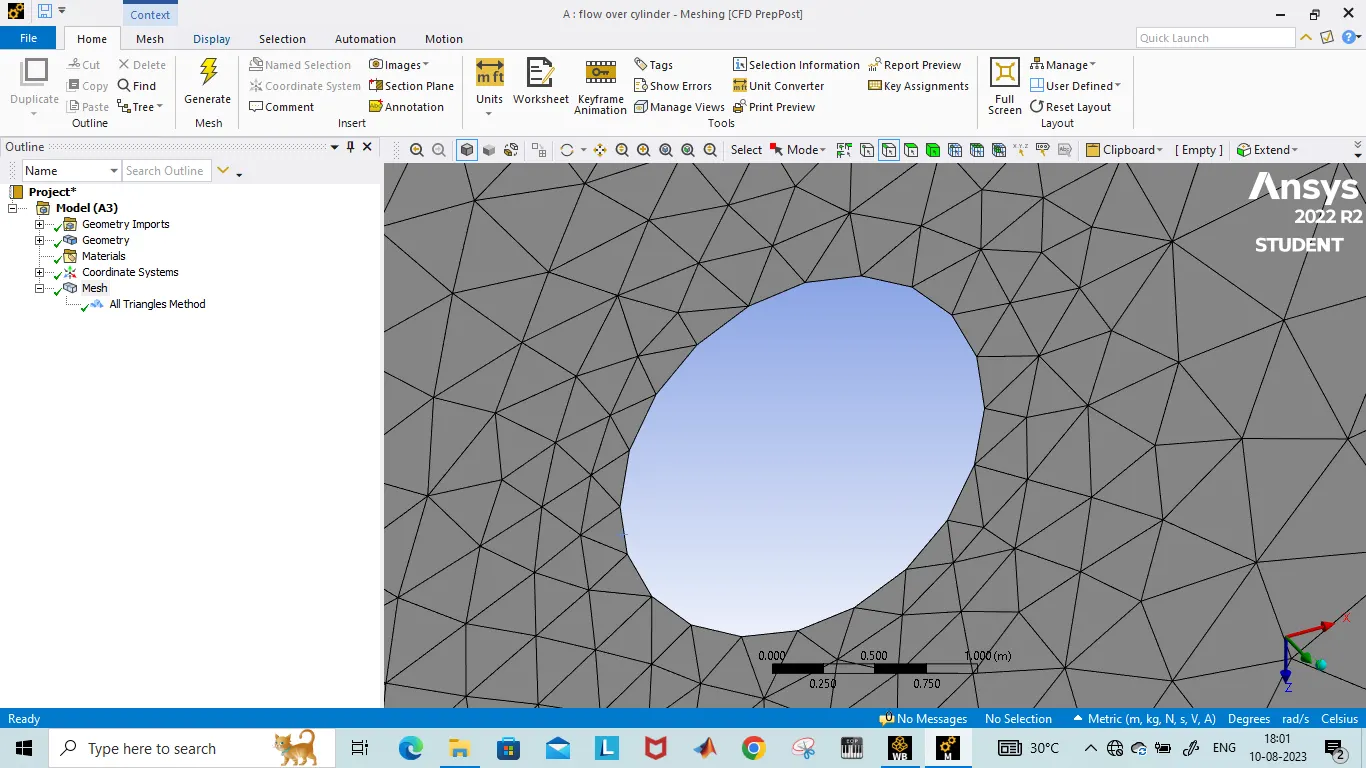
5)No of edges of circle turns to 36 to avoid polygon shape
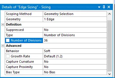
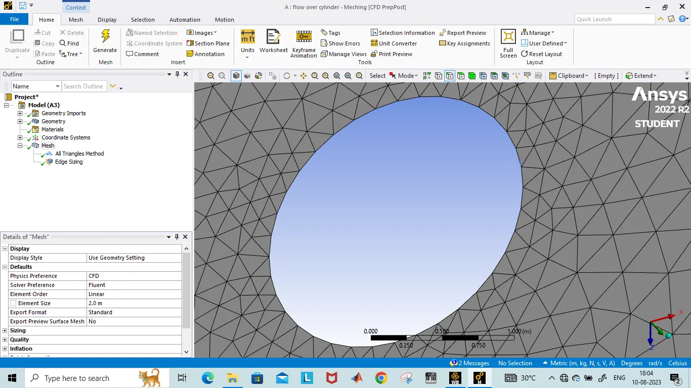
6)Resize of circle edges
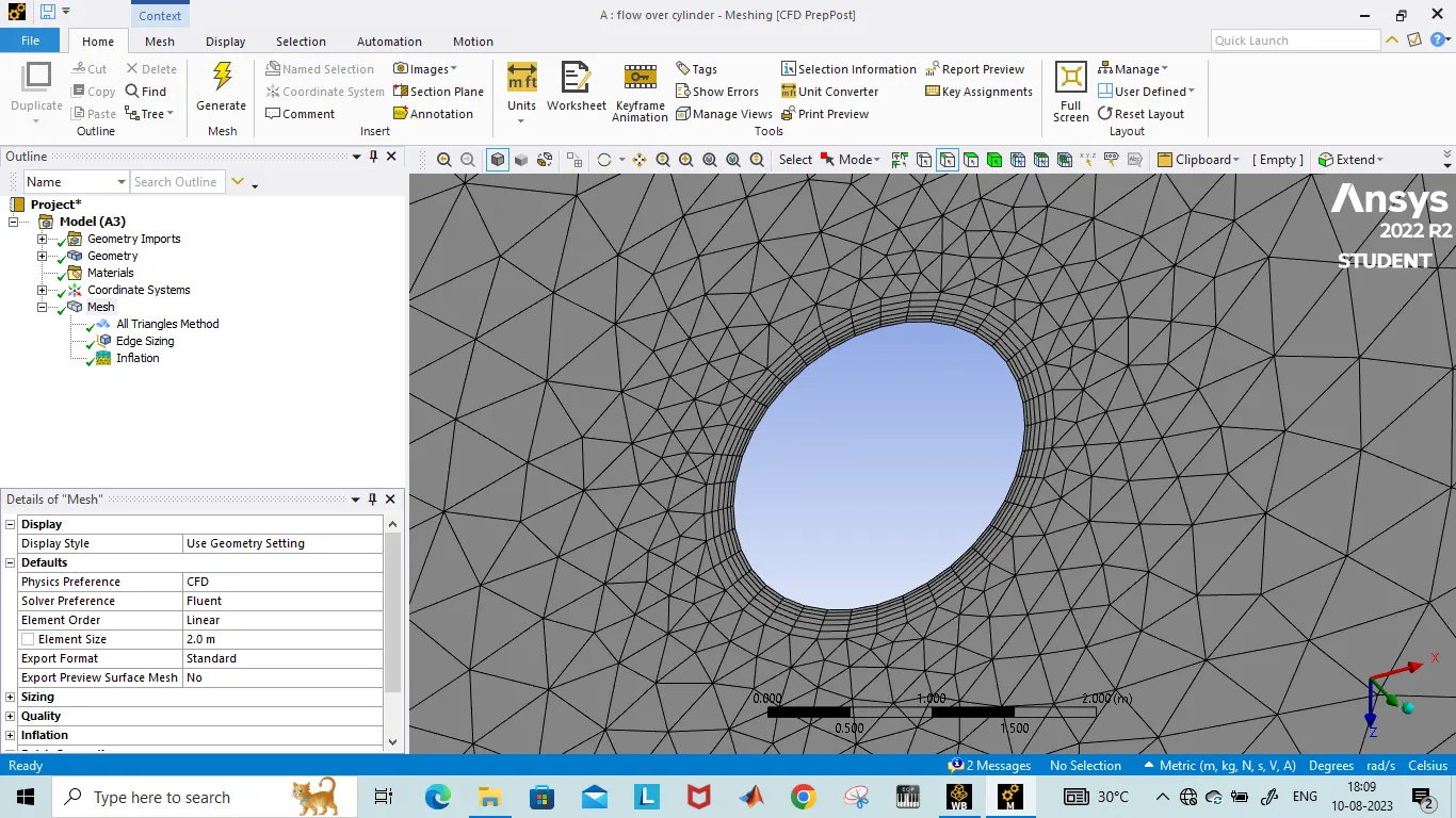
7)Inflation
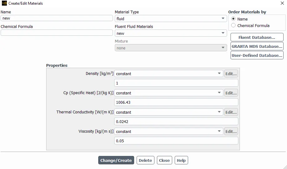
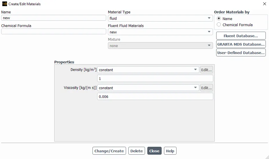
8)New material created
CASE 1A: STEADY STATE FLOW OVER CYLINDER
9)Contour plot of velocity for the viscous force of 0.05
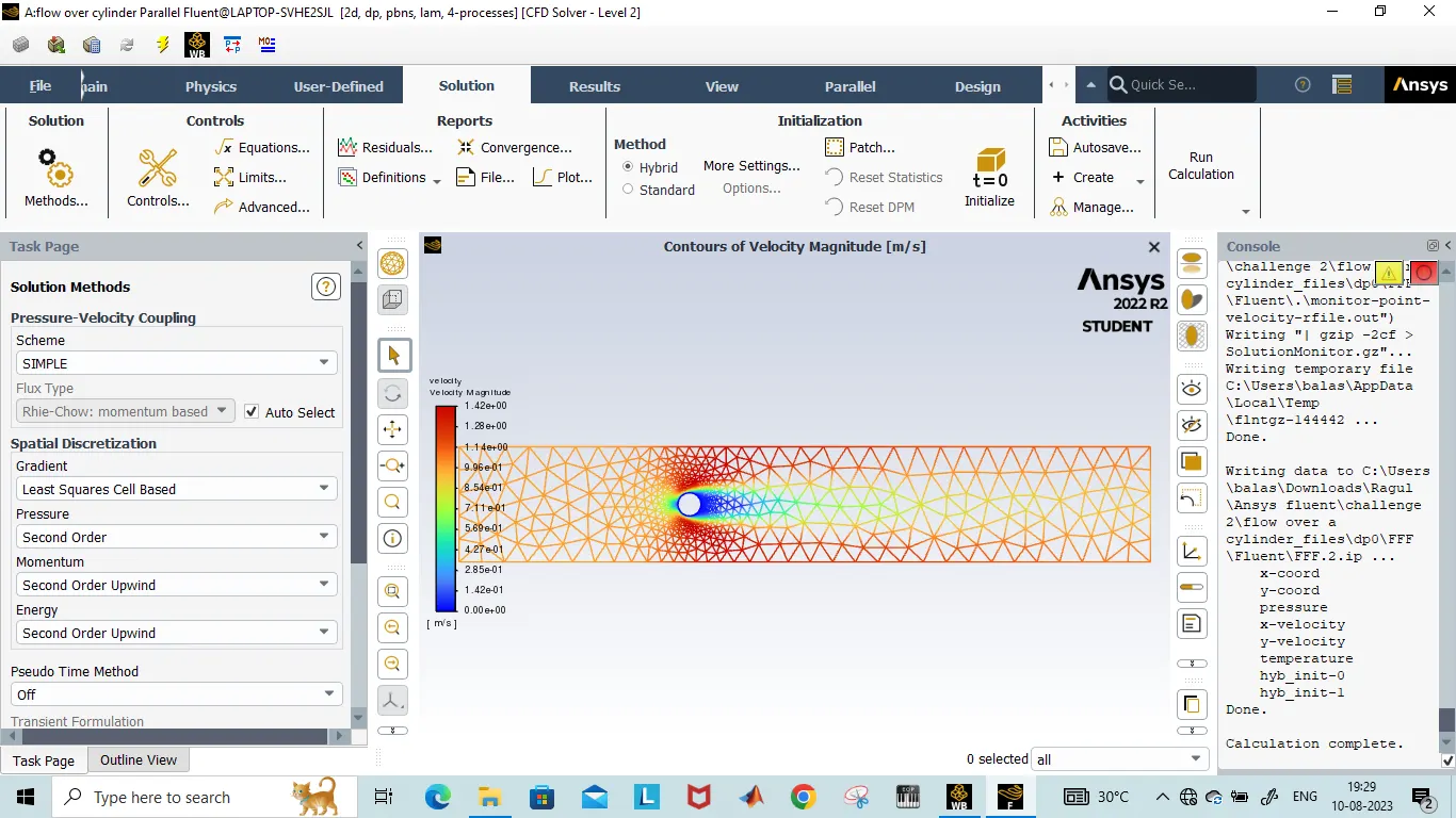
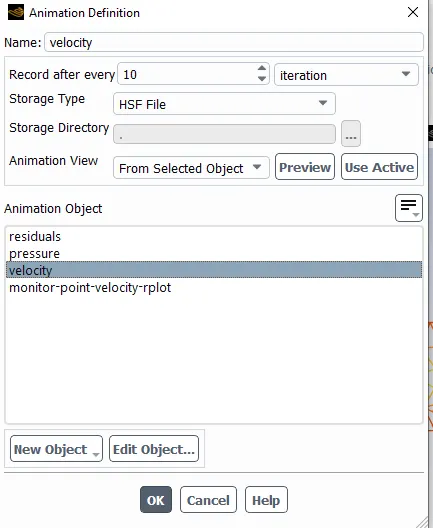
10)Animation setup created for velocity changes in the flow of fluid
11)Mesh element size reduced to 1m
12)Mesh element size reduced to 0.25m
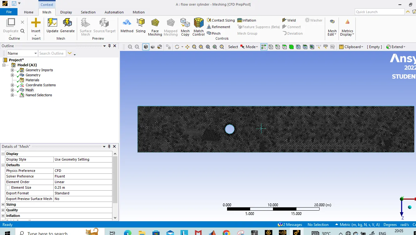
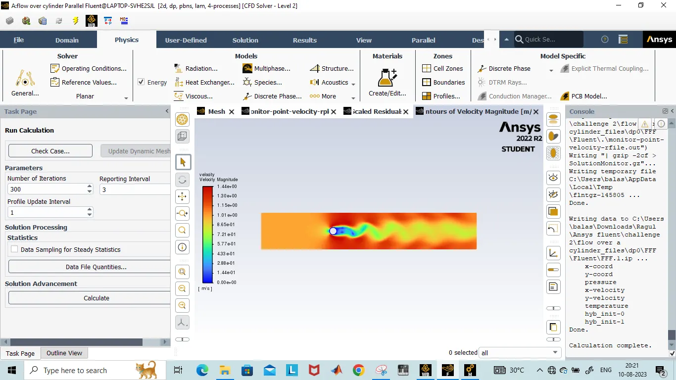
13)There is no vortex shedding create upto 0.25m mesh element length.So decided to reduce the viscous force for increasing the Reynolds number
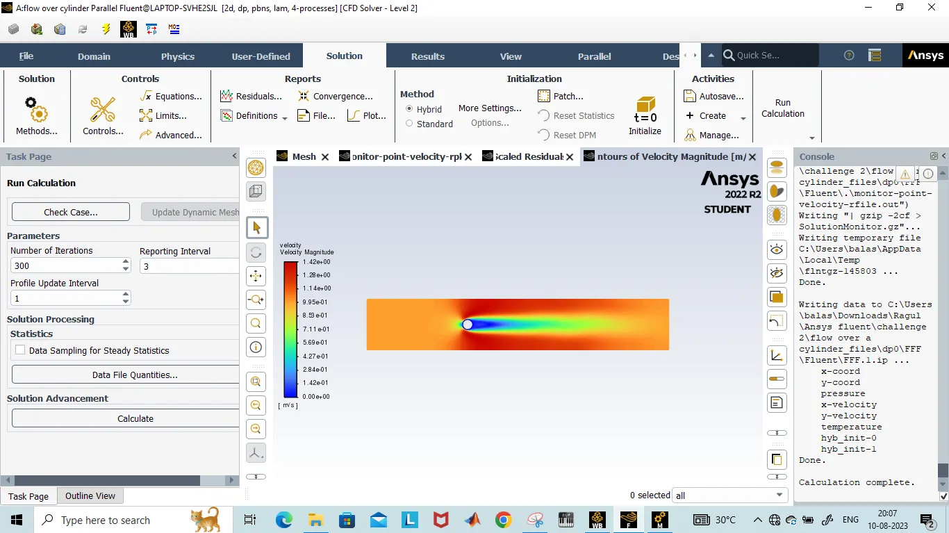
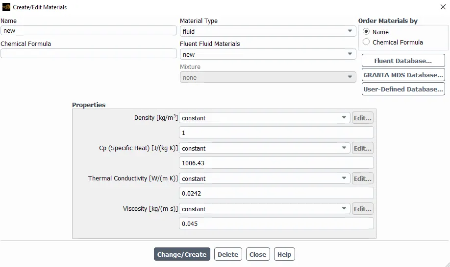
14)Viscous force is reduced to 0.045 and there is no creation vortex shedding
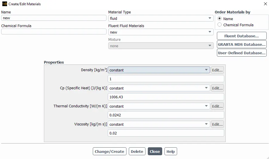
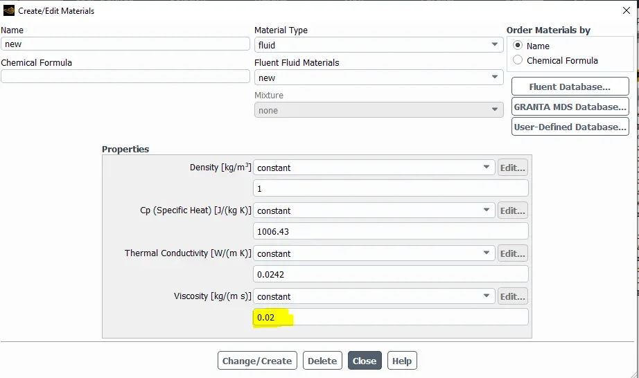
15)Now the viscous force is reduced 0.02
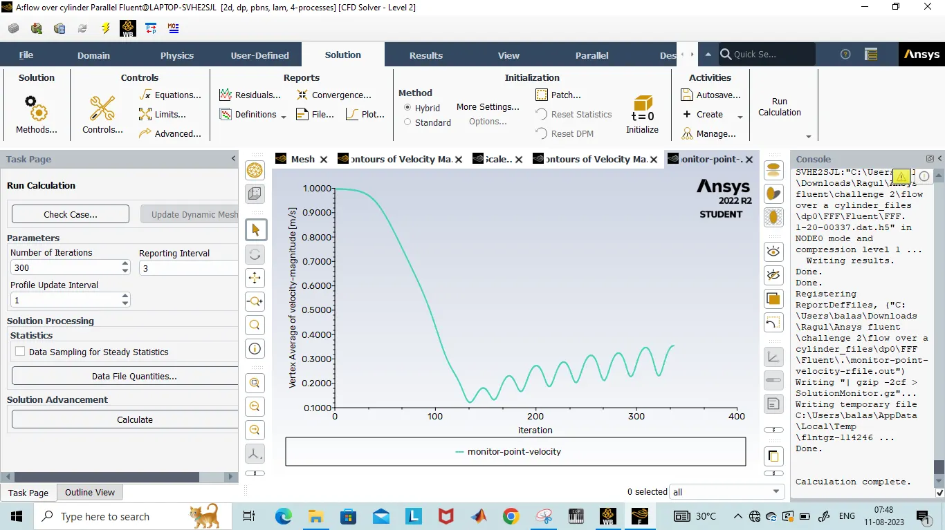
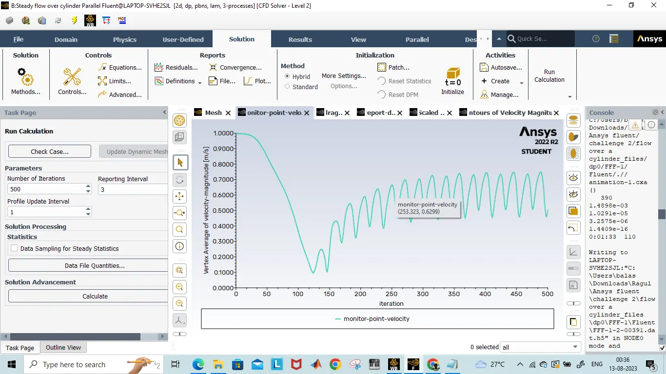
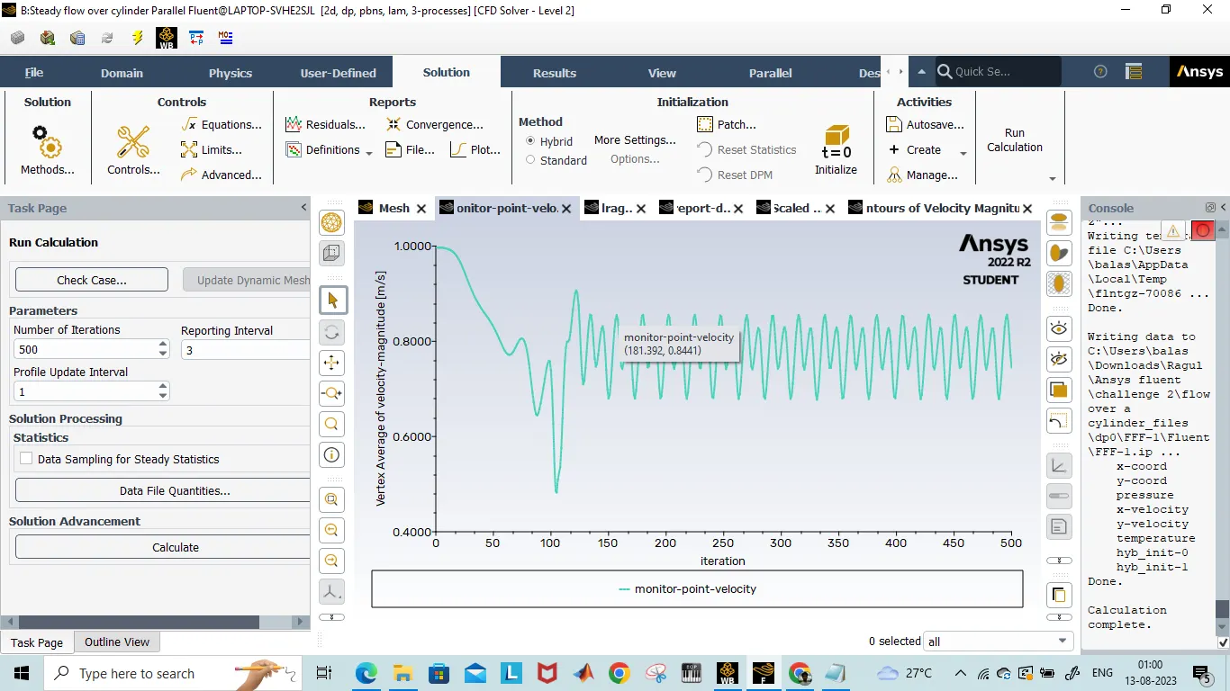
16)Monitor point is created at the distance of 8m from the centre of the cylinder to measure the velocity.Here the velocity graph there is oscillation in the velocity after 130 iteration
CASE 1B: UNSTEADY STATE(TRANSIENT) FLOW OVER CYLINDER
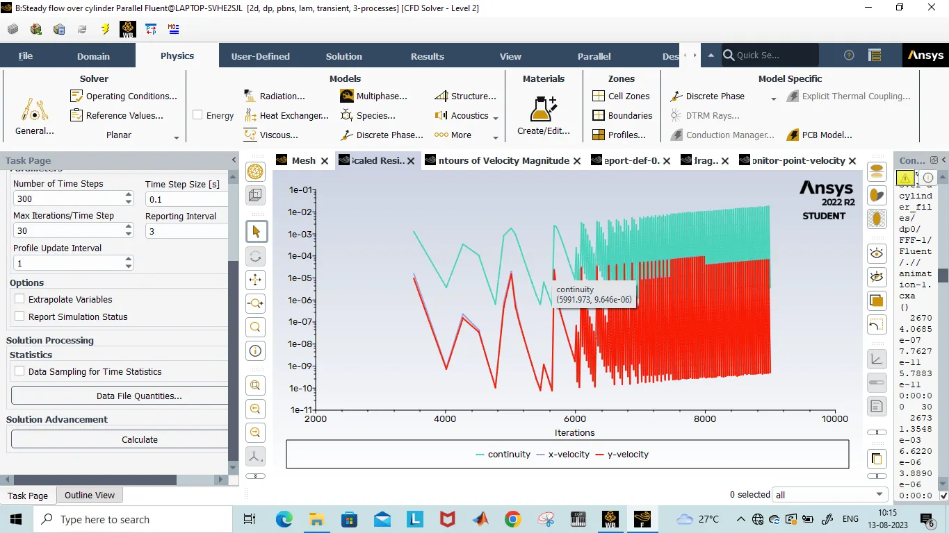
1)Simulating the series of plots for obtaining vortex shedding for unsteady flow. Varying the viscous force from high to small for increasing the reynolds number. At finally I got the vortex shedding of fluid above the reynolds number of 300
2)Residuals for unsteady flow
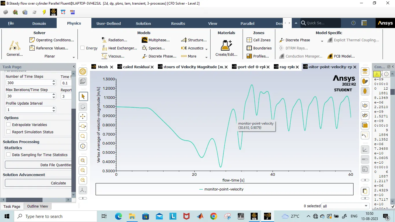
3)Vortex average shedding at Monitor point velocity for transient flow
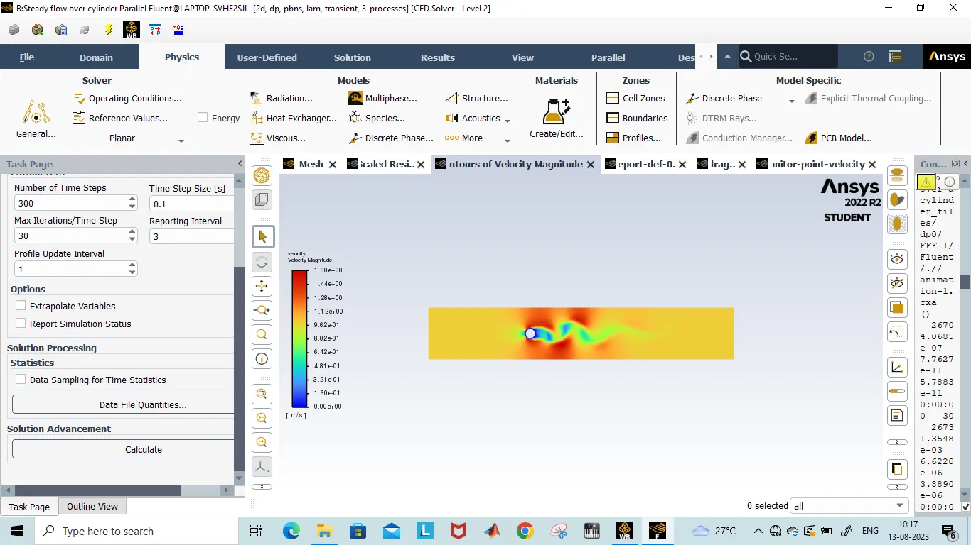
4)Contour velocity flow for transient flow
CASE 2: Simulation over cylinder with steady solver for Reynold number of 10,1000,10000,100000
For getting the given reynolds number, here use the imaginary value of viscous force.
| Density | 1 | kg/m^3 |
| Characteristic Length | 2 | m |
| Flow velocity | 1 | m/s |
| Reynolds Number | Viscous force | Unit |
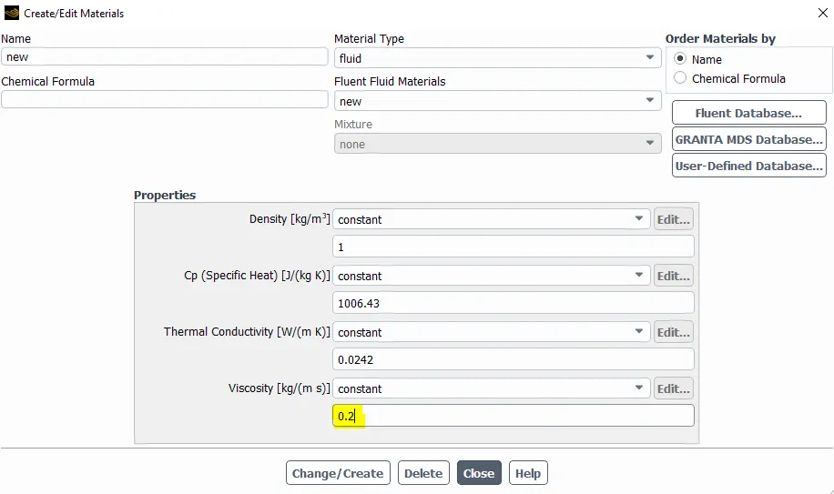
| 10 | 0.2 | kg/m/s |
| 100 | 0.02 | kg/m/s |
| 1000 | 0.002 | kg/m/s |
| 10000 | 0.0002 | kg/m/s |
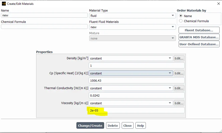
| 100000 | 0.00002 | kg/m/s |
A)Reynolds number of 10
A1)Reducing the viscous force
A2)Monitor point velocity checking
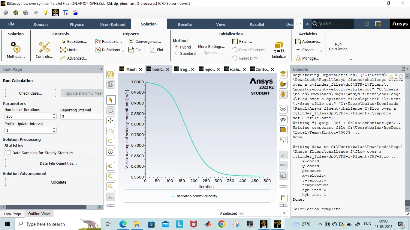
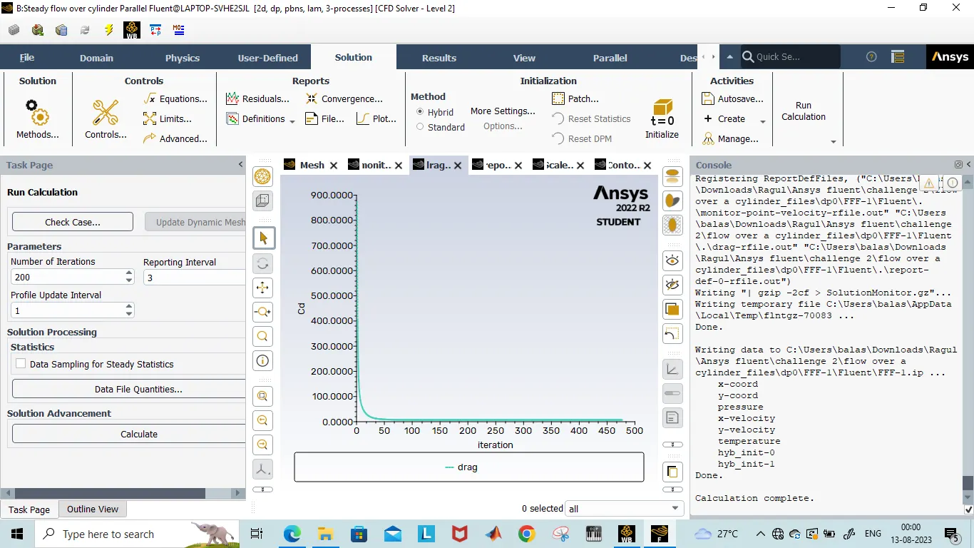
A3)Coefficient of drag
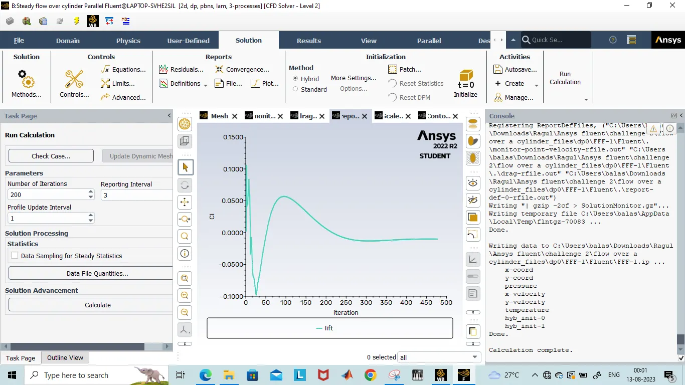
A4)Coefficient of lift
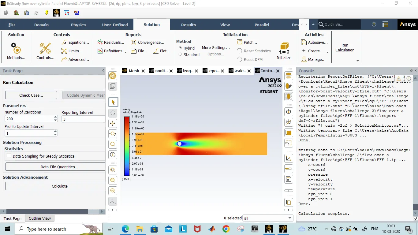
A5)Contour velocity
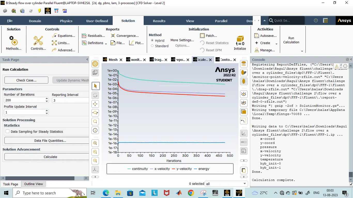
A6)Residuals
B)Reynolds number of 100
B1)Reducing viscous force
B2)Monitor point velocity
B3)Contour Velocity
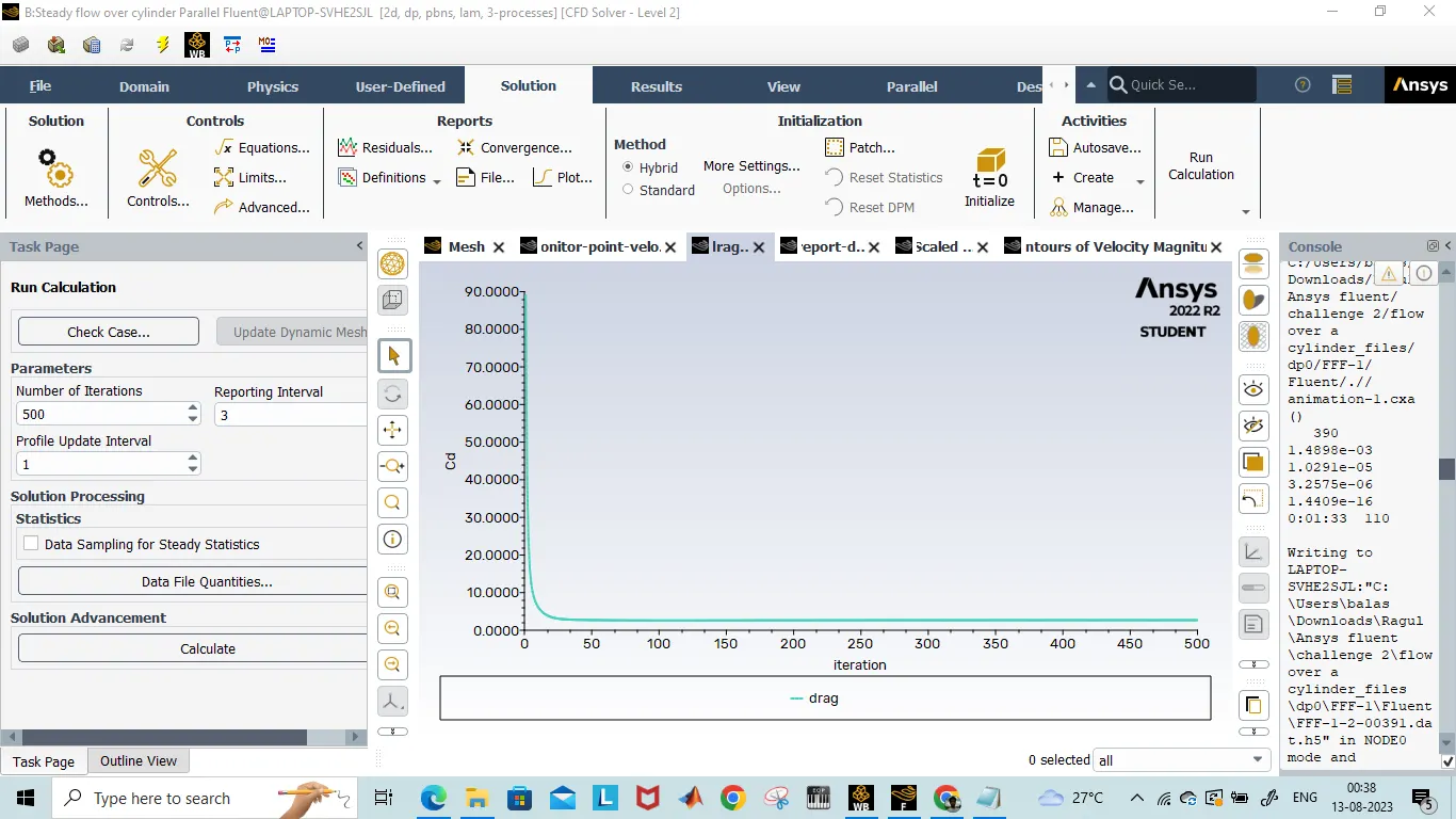
B4)Drag coefficent
B5)Lift Coefficient
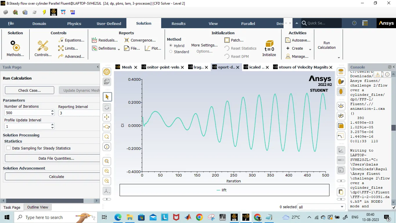
B6)Residuals
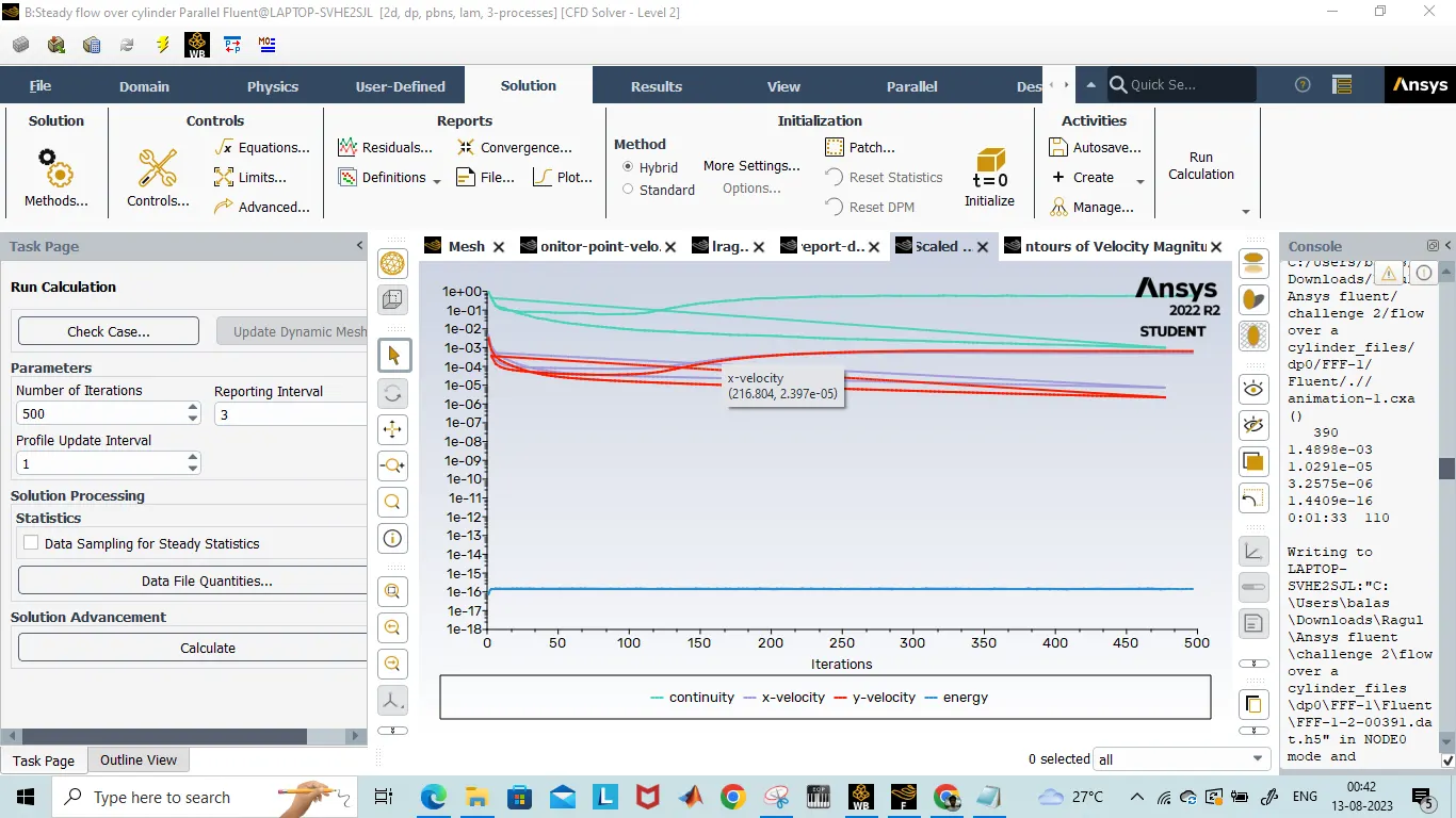
C)REYNOLDS NUMBER OF 1000
C1)Reducing visous force
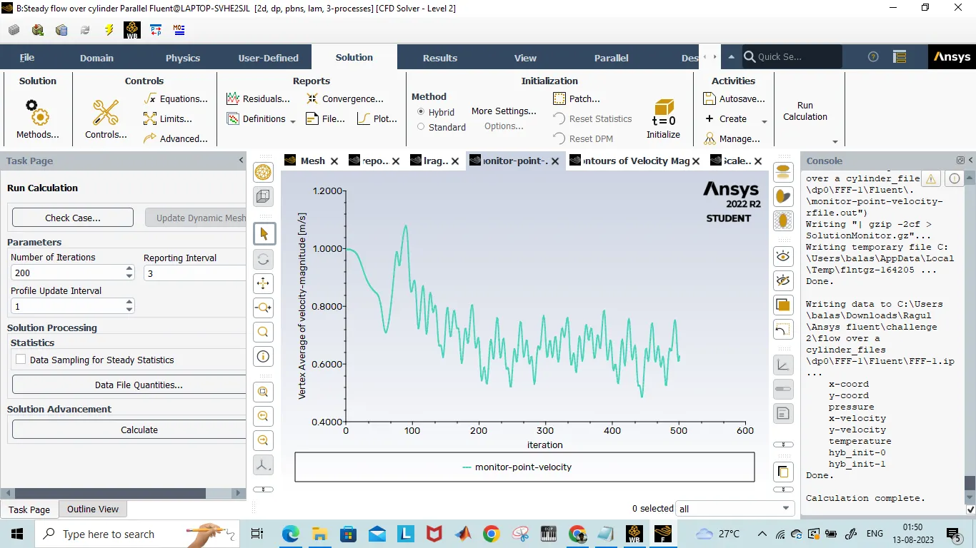
C2)Monitor point velocity
C3)Contour velocity
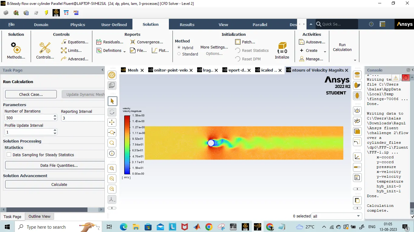
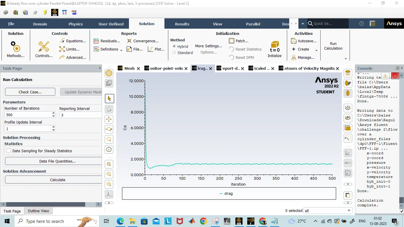
C4)Drag Coefficient
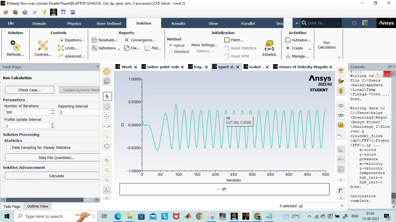
C5)Lift Coefficient
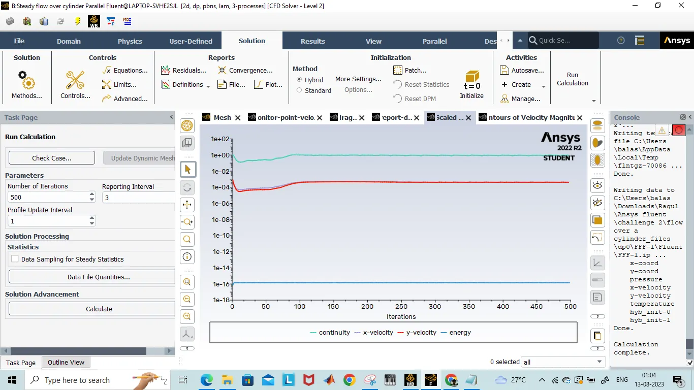
C6)Residuals
D)REYNOLDS NUMBER OF 10000
D1)Reducing viscous force
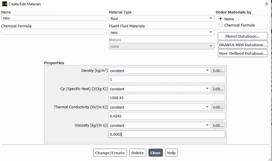
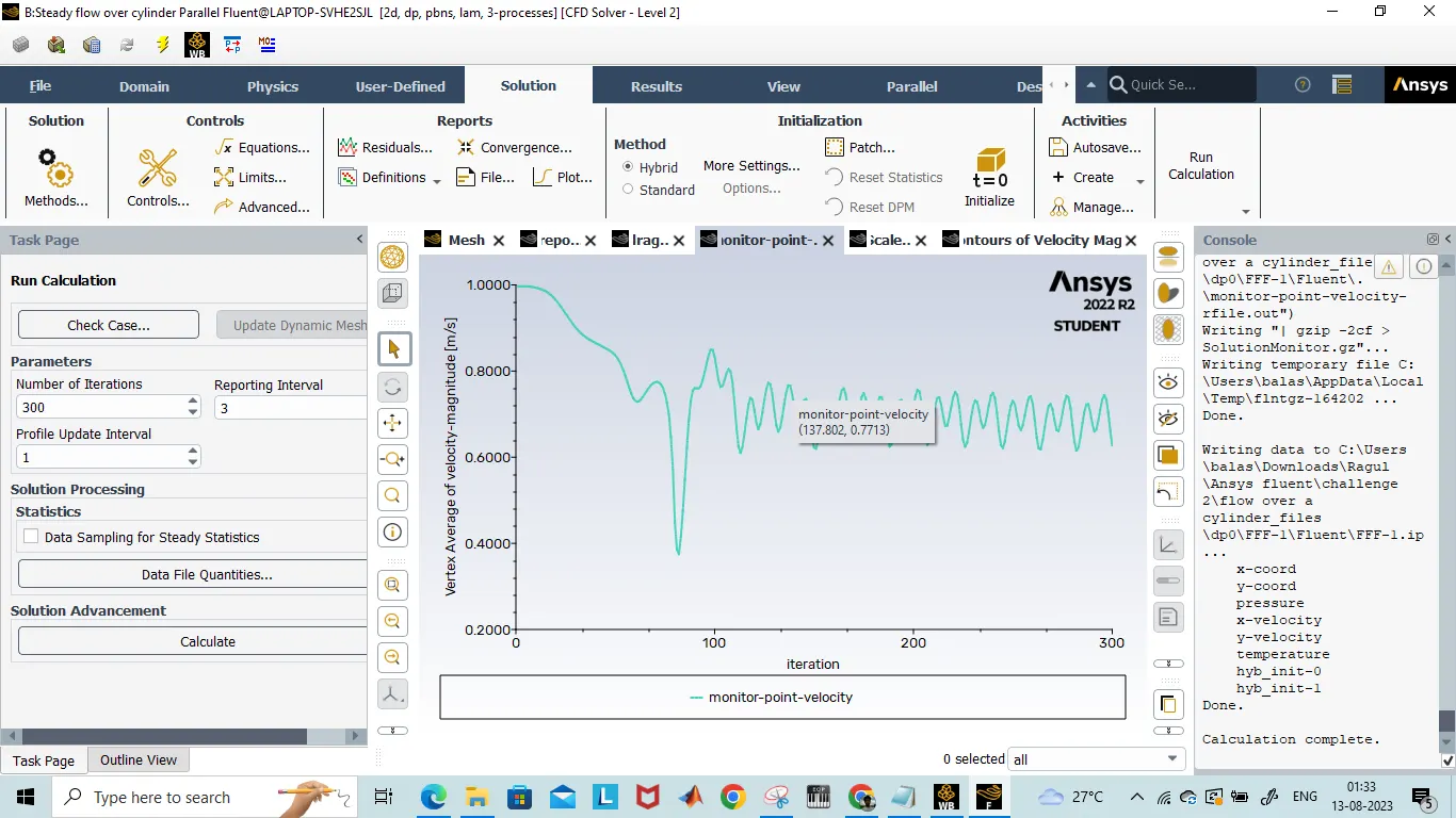
D2)Monitor point velocity
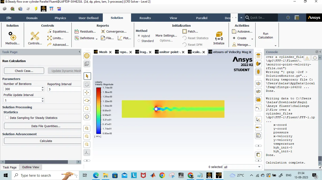
D3)Contour velocity
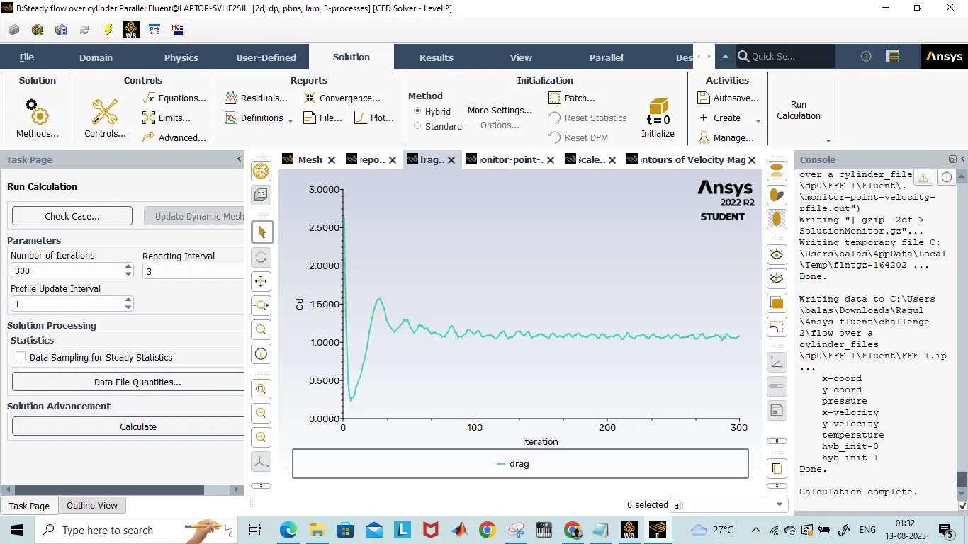
D4)Drag Coefficient
D5)Lift Coefficient
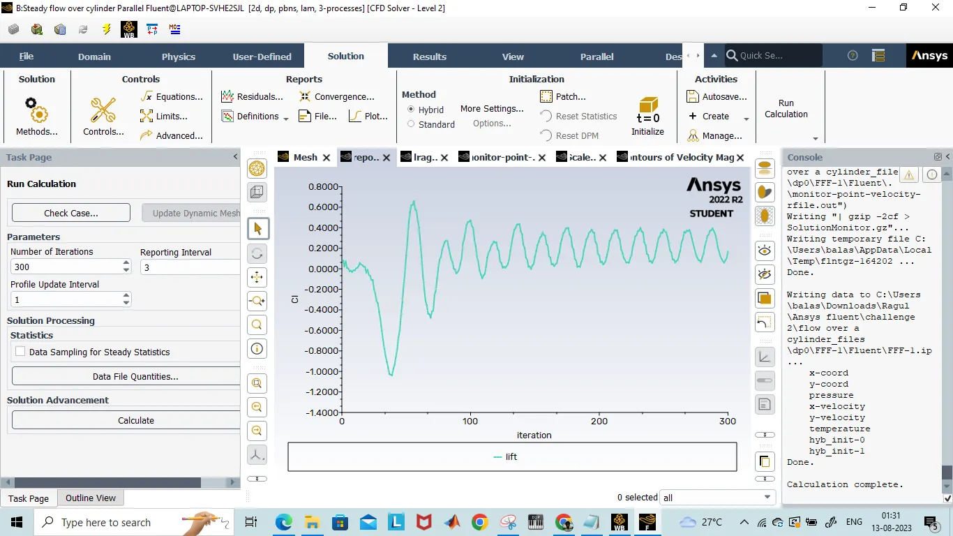
D6)Residuals
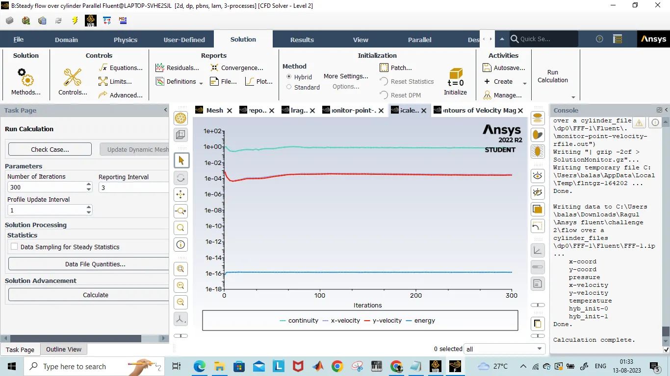
E)REYNOLDS NUMBER CHANGED TO 100000
E1)Reducing viscous force
E2)Monitor point velocity
E3)Contour Velocity
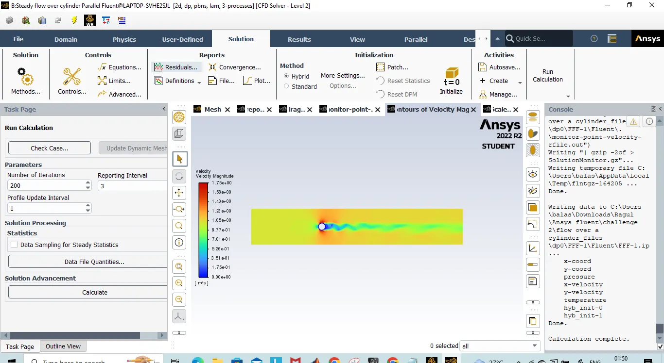
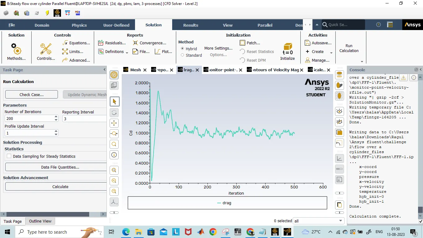
E4)Drag Coefficient
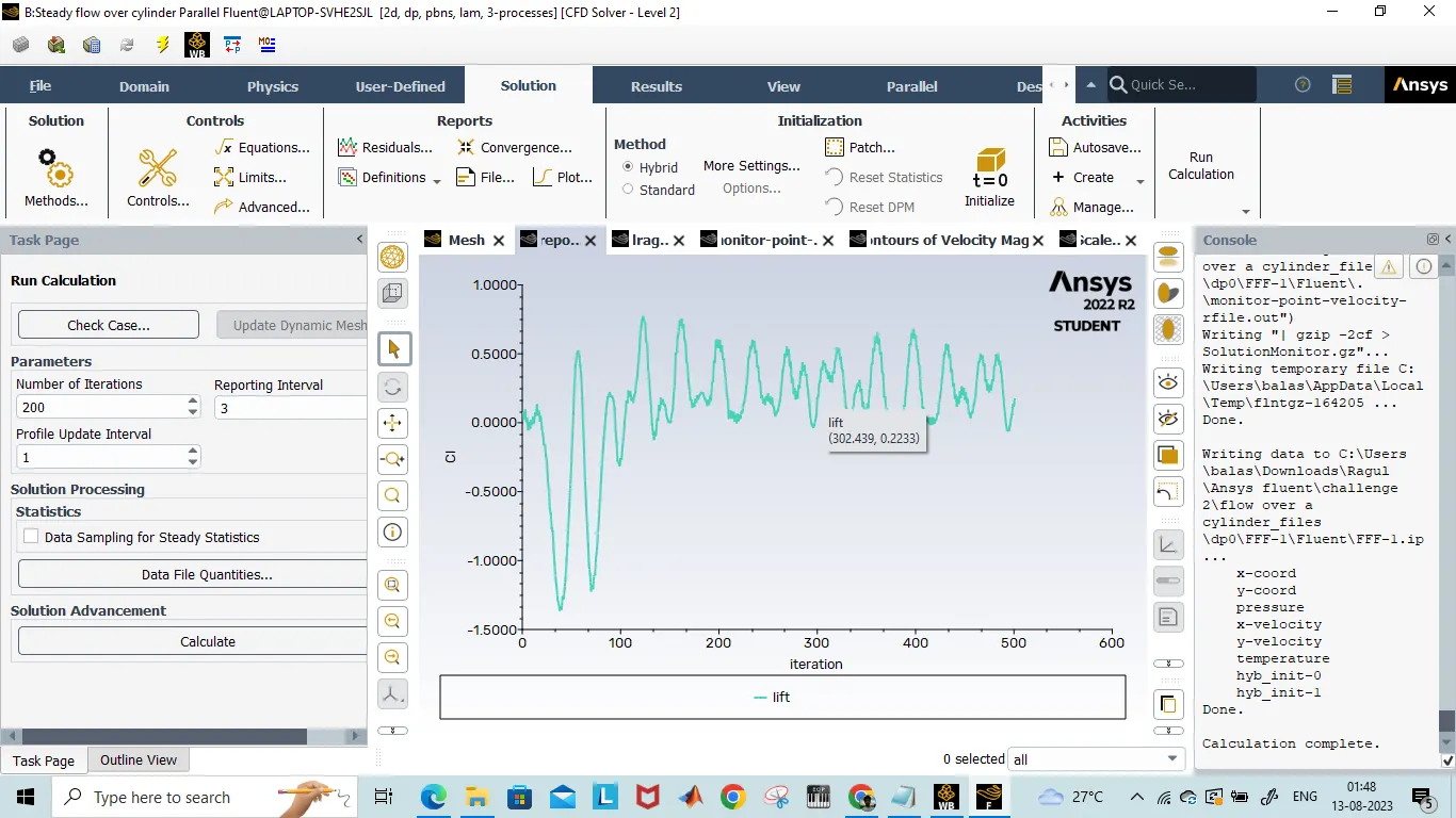
E5)Lift Coefficient
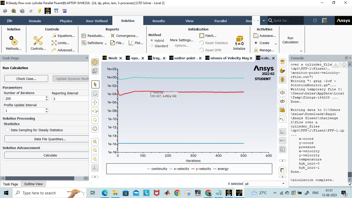
E6)Residuals
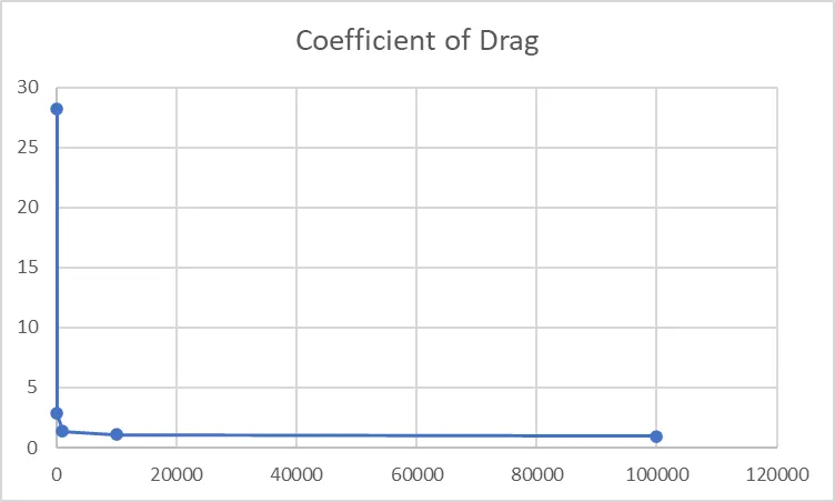
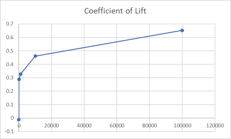
Comparison Table of Reynold number with Coefficient of Drag & Lift
| Reynolds Number | Coefficient of Drag | Coefficient of Lift |
| 10 | 28.169 | -0.011 |
| 100 | 2.834 | 0.287 |
| 1000 | 1.383 | 0.326 |
| 10000 | 1.087 | 0.461 |
| 100000 | 0.958 | 0.652 |
CONCLUSION
1) If we compare the data in the table, it is seen that as Reynolds number is increasing the coefficient of Drag is decreasing and coefficient of lift is increasing. This phenomenon is happening because when the Reynolds number gets increased the surface friction between fluid and cylinder is also increasing which causes the boundary layer to break before the flow separated hence the amount of drag get decreases and lift get increases.
2) As the Reynolds number increase, the wake region behind the cylinder is also increasing which results in a bigger domain area for further simulations.
3)The time & resources consumed by the transient solver is far more than the steady-state solver. In transient mode, more iterations are required to develop the proper physics of the flow. Because of that the transient simulation has taken more iteration with smaller time steps compared to the steady state.
4)The drag coefficient for the Re above 1000, is start fluctuating but periodic after one point which can be seen from the results images. So statistically, it is taken as constant.