Week 2 - Flow over a Cylinder.
Aim: To simulate the flow over the cylinder and to understand the vortex shredding phenomena over the cylindrical region.
Vortex Shedding: it is the phenomenon of the formation of a vortex across the cylindrical region due to the pressure difference at the front and top & bottom surface of the cylinder, and survives for a short span of time and is finally shredded, the vortex formation keeps repeating, as a result, it induces external force over such wake region of the cylinder.
Strouhal Number (SN): it is a dimensionless number, which is generally used to measure the shedding frequency (f);
SN=f*D/V
Where, D= dia of cylinder, V= free stream velocity
Procedure:
Geometry Formation (2D space claim):
Meshing: (using Insert method, inflation method for body fitted mesh)
Setting Up Physics:
Material Used: Air-new (density=1.2kg/m^3, viscosity=.04 kg/(m-s))
Viscous model : laminar
|
CASE |
|
|
Density (kg/m^3) |
1.2 |
|
Viscosity (kg/(m-s)) |
0.4 |
|
Diameter (m) |
2 |
|
Reynold No. |
100 |
|
Velocity (m/s) |
16.66666667 |
Part I: Steady and Unsteady flow over cylinder, and calculation of stouhal no. for reynold no. 100
Steady State:
Solver: pressure based steady solver
Initialization type: hybrid
No. of iteration: 500
Unsteady State:
Solver: pressure based unsteady solver
Initialization type: hybrid
Time step size: 0.2s
No. of timestep: 1200
Result:
Steady State:
Convergence Plot:
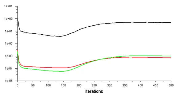
gets converged around 300 iterations
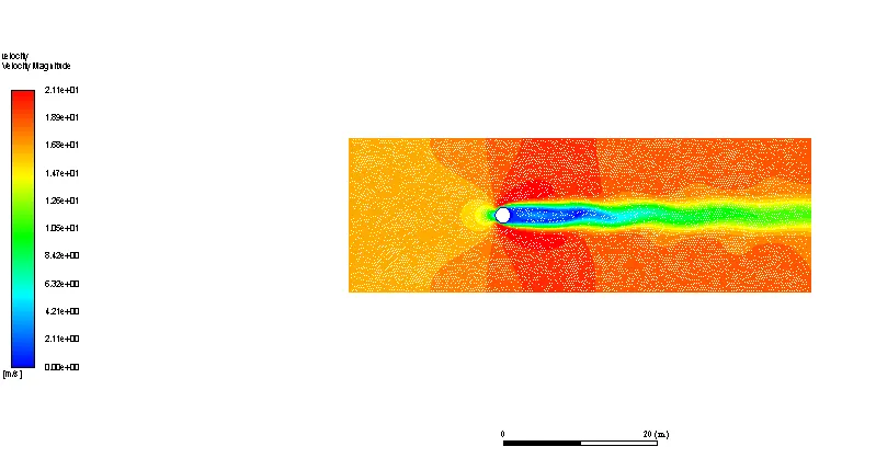
Velocity Contour:
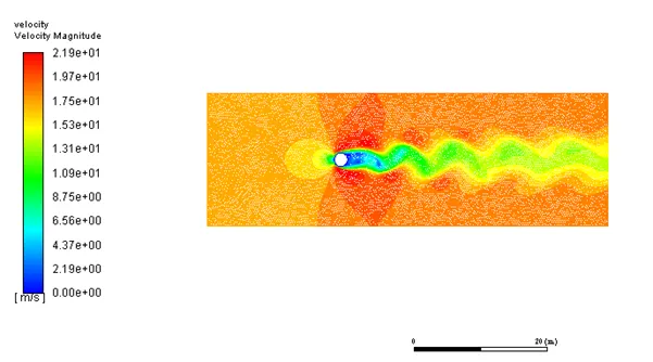
depicts max velocity of 21.9 m/s which is at the top and bottom surface, and gets low around back region, leads to the geneation of wake.
Pressure Contour:
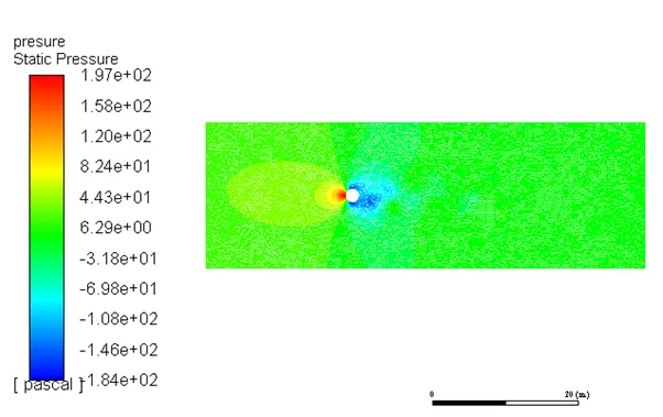
indicate max pressure of 197 Pa at the front surace of cylinder as whole kinetic energy of the fluid converted to pressure energy (stagnation Point).
Velocity Coutour:
Pressure Contour:
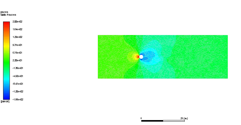
both velocity and pressure contour are same as Steady state.
Vertex Plot:
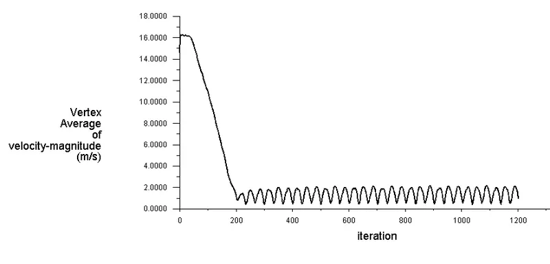
indicates vortex formation starts around 220 iteration, which means after 44 seconds
Unsteady state:
Convergence Plot:
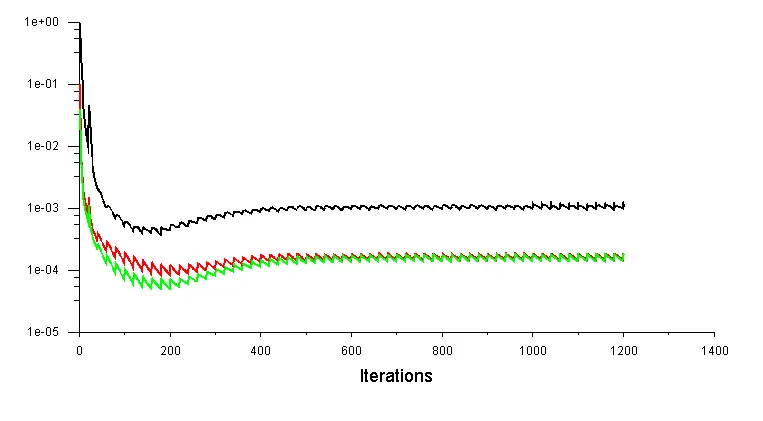
gets converged around 600 Iteration.
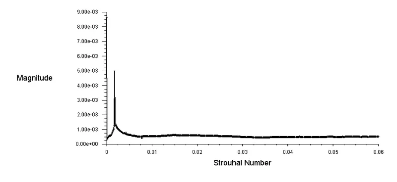
Stouhal No.: 0.03
Solution Of Part II:
|
CASE I |
|
|
Density (kg/m^3) |
1.2 |
|
Viscosity (kg/(m-s)) |
0.4 |
|
Diameter (m) |
2 |
|
Reynold No. |
10 |
|
Velocity (m/s) |
1.666666667 |
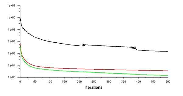
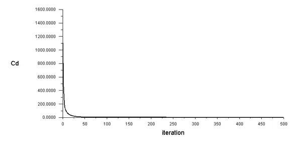
Convergence Plot:
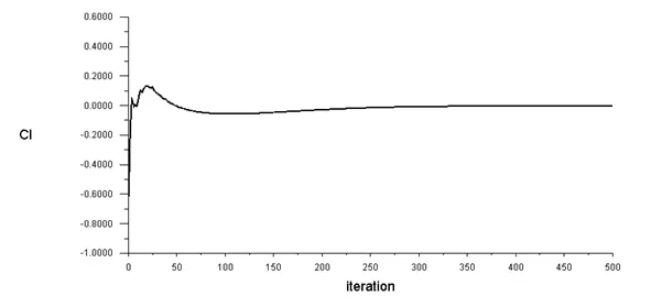
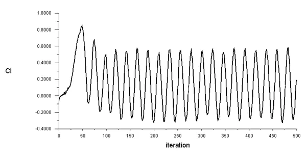
Coefficient Of Lift Plot:
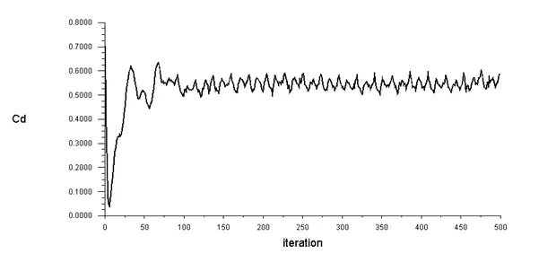
Coefficient Of Drag Plot:
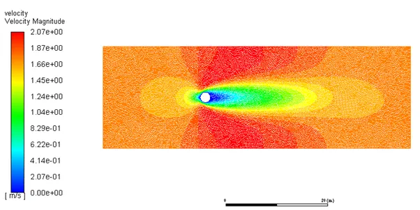
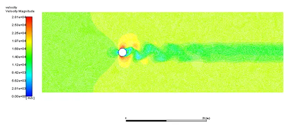
Velocity Contour:
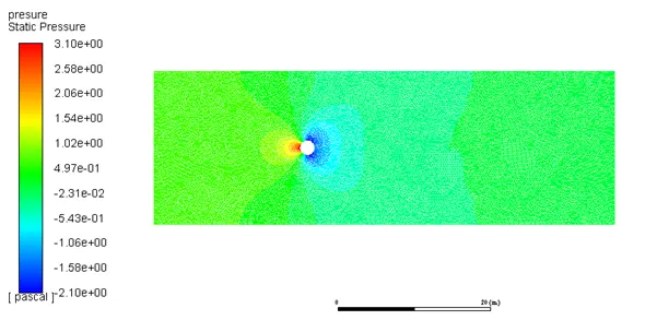
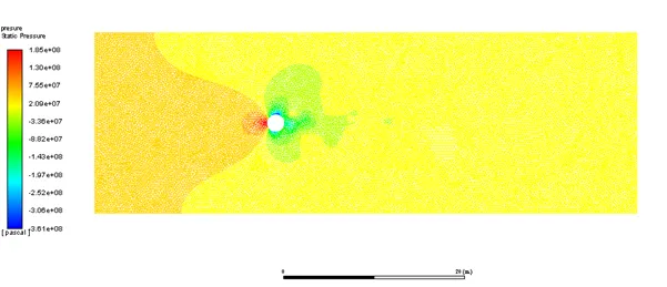
Pressure Contour:
|
CASE 2 |
|
|
Density (kg/m^3) |
1.2 |
|
Viscosity (kg/(m-s)) |
0.4 |
|
Diameter (m) |
2 |
|
Reynold No. |
100 |
|
Velocity (m/s) |
16.66666667 |
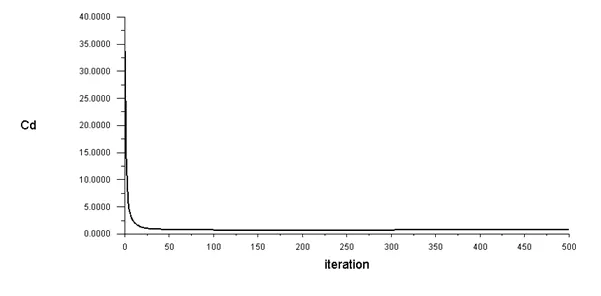
Convergence Plot:
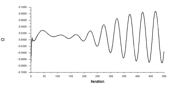
Coefficient Of Lift Plot:
Coefficient Of Drag Plot:
Velocity Contour:
Pressure Contour:
|
CASE 3 |
|
|
Density (kg/m^3) |
1.2 |
|
Viscosity (kg/(m-s)) |
0.4 |
|
Diameter (m) |
2 |
|
Reynold No. |
1000 |
|
Velocity (m/s) |
166.6666667 |
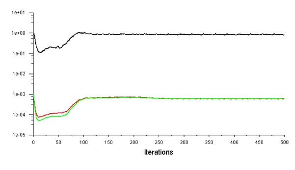
Convergence Plot:
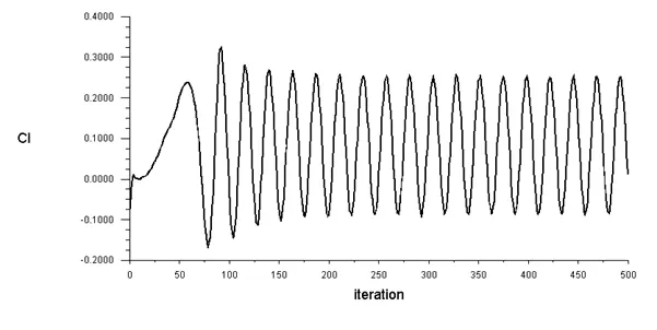
Coefficient Of Lift Plot:
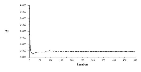
Coefficient Of Drag Plot:
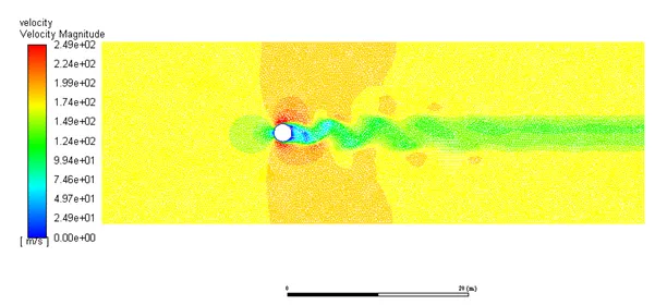
Velocity Contour:
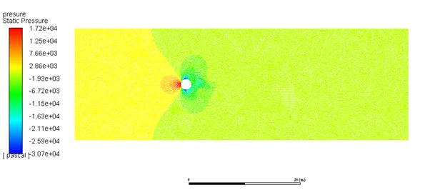
Pressure Contour:
|
CASE 4 |
|
|
Density (kg/m^3) |
1.2 |
|
Viscosity (kg/(m-s)) |
0.4 |
|
Diameter (m) |
2 |
|
Reynold No. |
10000 |
|
Velocity (m/s) |
1666.666667 |
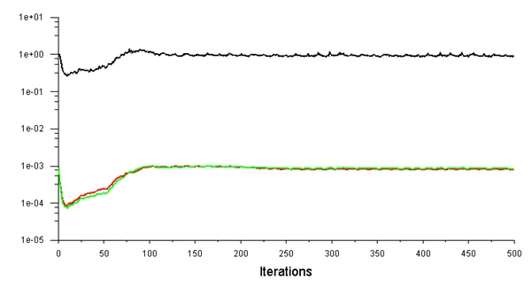
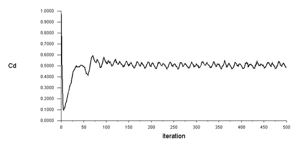
Convergence Plot:
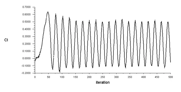
Coefficient Of Lift Plot:
Coefficient Of Drag Plot:
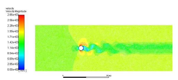
Velocity Contour:
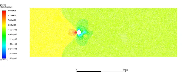
Pressure Contour:
|
CASE 5 |
|
|
Density (kg/m^3) |
1.2 |
|
Viscosity (kg/(m-s)) |
0.4 |
|
Diameter (m) |
2 |
|
Reynold No. |
100000 |
|
Velocity (m/s) |
16666.66667 |
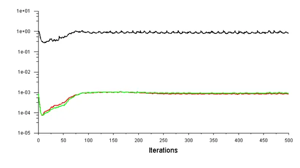
Convergence Plot:
Coefficient Of Lift Plot:
Coefficient Of Drag Plot:
Velocity Contour:
Pressure Contour:
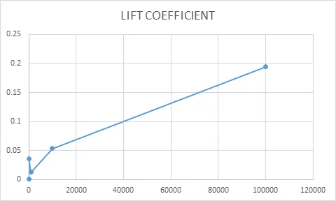
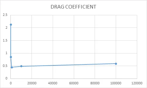
Following are the variation of Cd and Cl wrt Reynold No.
|
CASE |
REYNOLD NO. |
LIFT COEFFICIENT |
DRAG COEFFICIENT |
|
1 |
10 |
0.000537202 |
2.1210989 |
|
2 |
100 |
0.035810273 |
0.85015816 |
|
3 |
1000 |
0.012462425 |
0.44456731 |
|
4 |
10000 |
0.053153393 |
0.48270197 |
|
5 |
100000 |
0.19410769 |
0.58504671 |