Week 2 - Flow over a Cylinder.

FLOW OVER A CYLINDER

Aim: Simulation of flow over the cylinder and observing the Karman Vortex phenomenon

Objective:

Prepare the computational domain for the given problem of an external fluid flow simulation.

Understand the formation of vortices around a bluff body, deduce the drag and lift coefficient and study the effect of Reynolds number on the vortices so formed.

Understand the principle of Karman vortex street and evaluate Strouhal number for the given flow over the cylinder.

INTRODUCTION:

Computational fluid dynamics (CFD) is a tool to solve fluid flow problems; it has become an alternative to experiments in a lot of cases. In many ways CFD tools can be superior to experimentation. Flow over a cylinder is a classical problem for understanding the flow over an obstacle. The geometry of the cylinder is simple and allows us to understand all the complexities that occur and turbulence for different Reynolds Numbers. Reynolds Number helps us to understand the flow patterns of the different fluid flow situations. The different range of Reynolds Numbers represents different flow patterns. At low Reynolds Numbers, the flow pattern is observed to be Laminar i.e., Smooth, Constant fluid motion. At higher Reynolds Numbers the flow pattern is observed to be Turbulent i.e., Chaotic eddies, Vortices, and Flow instabilities. In this project, we will try to understand the variation of velocity and pressure in certain flow directions for different Reynolds Numbers by simulating it with proper boundary conditions, Mesh sizing, Convergence criteria using SolidWorks Flow Simulation.

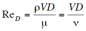
Reynolds number is a dimensionless quantity that is used to determine the type of flow pattern as laminar or turbulent while flowing through a pipe. Reynolds number is defined by the ratio of inertial forces to that of viscous forces.

Where,

• R_e is the Reynolds number
• ρ is the density of the fluid
• V is the velocity of flow
• D is the pipe diameter
• μ is the viscosity of the fluid

If the Reynolds number calculated is high (greater than 2000), then the flow through the pipe is said to be turbulent. If Reynolds number is low (less than 2000), the flow is said to be laminar. Numerically, these are acceptable values, although in general the laminar and turbulent flows are classified according to a range. Laminar flow falls below Reynolds number of 1100 and turbulent falls in a range greater than 2200.

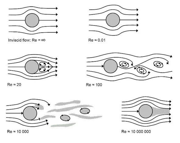
Flow over a cylinder is important in many industrial application like cooling of iron or cylindrical pipe

Circular pipes have more application in heat exchanger. High temperature flue gases flow over a circular cylinder in a cross flow.

In fluid dynamics a Karman vortex street (or a von Kármán vortex street) is a repeating pattern of swirling vertices, caused by a process known as vertex shedding, which is responsible for the unsteady separation of flow of a fluid around blunt bodies.

It is named after the engineer and fluid dynamitist Theodore von Karman, and is responsible for such phenomena as the "singing" of suspended telephone or power lines and the vibration of a car antenna at certain speeds. Mathematical modeling of von Kármán vortex street can be performed using different techniques including but not limited to solving the full Navier-Stokes equations with k-epsilon, SST, k-omega and Reynolds stress, and large eddy simulation (LES) turbulence models and numerically solving some dynamic equations such as the Ginzburg-Landau equation.

A vortex street will form only at a certain range of flow velocities, specified by a range of Reynolds Number (Re), typically above a limiting Re value of about 90. The (global) Reynolds number for a flow is a measure of the ratio of inertial to viscous forces in the flow of a fluid around a body or in a channel, and may be defined as a non-dimensional parameter of the global speed of the whole fluid flow:

R_(e_L )= UL/v_0

{\displaystyle \mathrm {Re} _{L}={\frac {UL}{\nu _{0}}}}

where:

• {\displaystyle U}U is the free stream flow speed
• {\displaystyle L}L is a characteristic length parameter of the body or channel
• {\displaystyle \nu _{0}}v_0 is the free stream kinematic viscosity parameter of the fluid, which in turn is the ratio:

{\displaystyle \nu _{0}={\frac {\mu _{0}}{\rho _{0}}}}

v_0= μ_0/ρ_0

between:

• {\displaystyle \rho _{0}} is the free stream fluid dynamic viscosity
• {\displaystyle \mu _{0}} is the reference fluid density.

Formula:

{\displaystyle {\text{St}}=0.198\left(1-{\frac {19.7}{{\text{Re}}_{d}}}\right)\ }

St=0.198(1-19.7/R_(e_d ) )

where:

{\displaystyle {\text{St}}={\frac {fd}{U}}}

St = f*d/U

• f = vortex shedding frequency.
• d = diameter of the cylinder
• U = flow velocity.

CASE 1:

In this part results for, for Re 100, steady & unsteady simulation will be presented.

For steady state simulation:

Viscosity: 0.02 Kg/m-s

Flow velocity: 2 m/s

Density: 1 Kg/m^3

Calculating Strouhal Number for Re 100 we get

Strouhal Number of 0.1589 ≈ 0.16.

Steady state simulation of drag coefficient, lift coefficient, monitor pint velocity, pressure contour, residuals, Strouhal number & velocity contour are presented below,

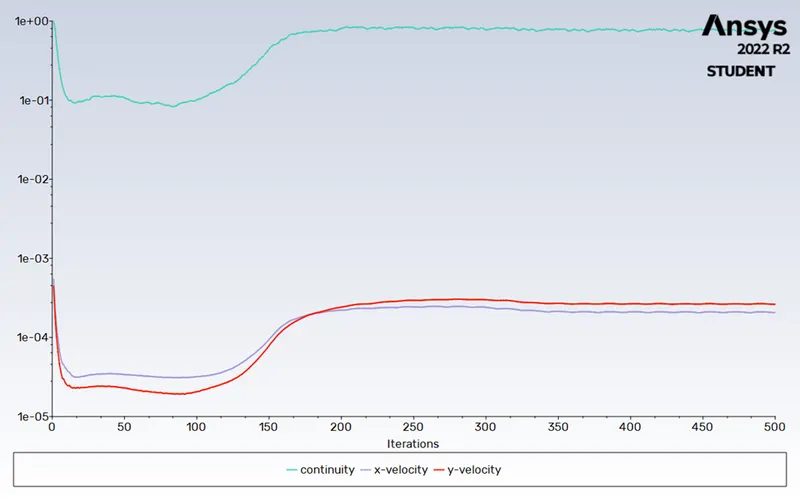
RESIDUAL PLOT:

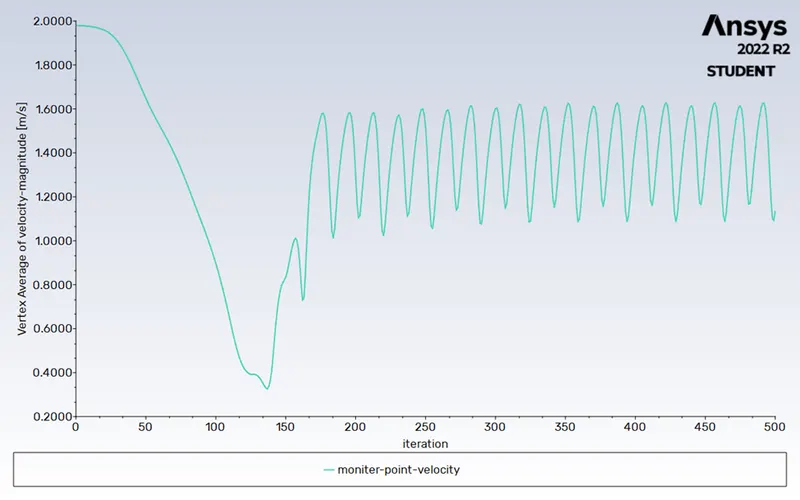
FLOW VELOCITY PLOT:

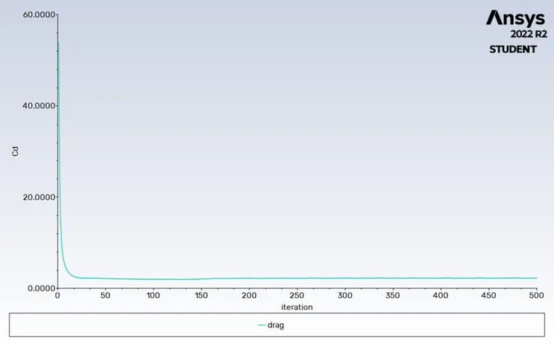
DRAG COEFFICIENT:

LIFT COEFFICIENT:

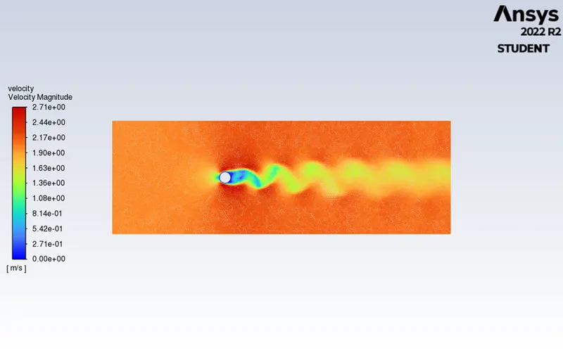
VELOCITY MAGNITUDE:

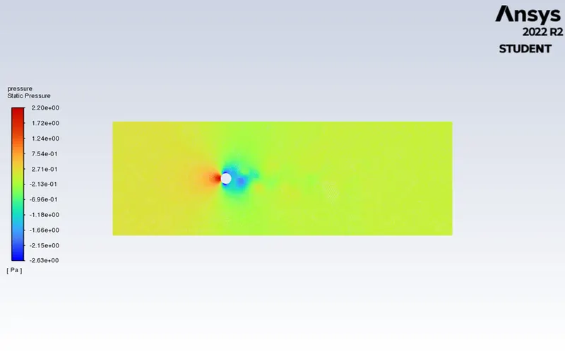
STATIC PRESSURE:

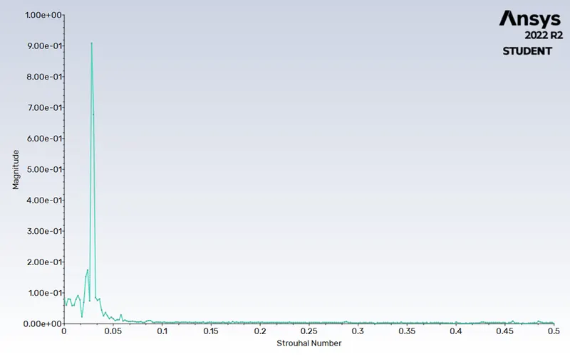
STROUHAL NUMBER:

UNSTEADY STATE SIMULATION IMAGES:

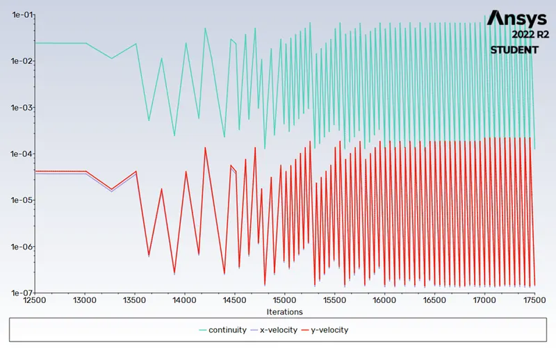
RESIDUAL:

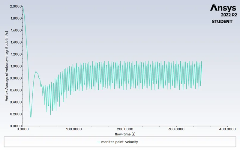
VELOCITY MAGNITUDE:

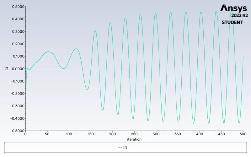
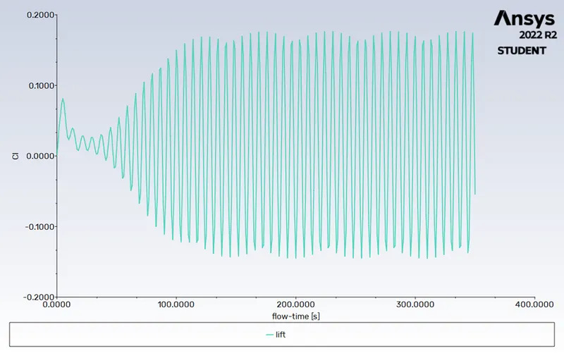
LIFT COEFFICIENT:

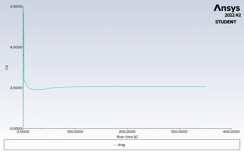
DRAG COEFFICIENT:

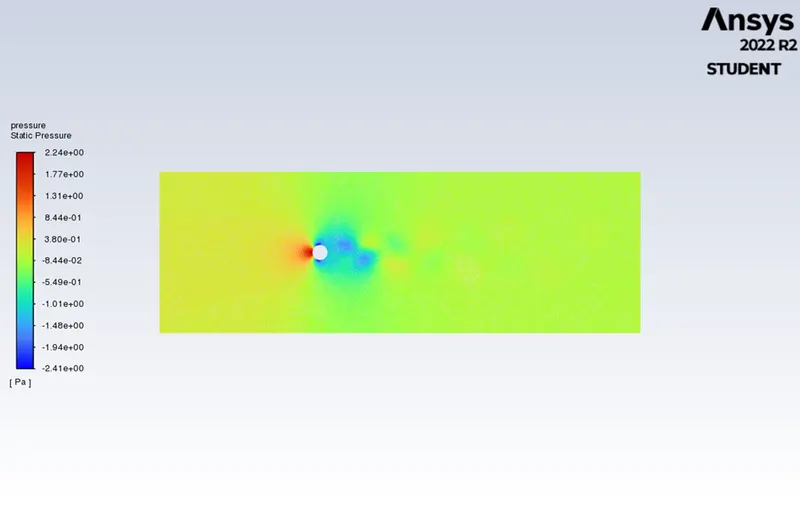
PRESSURE:

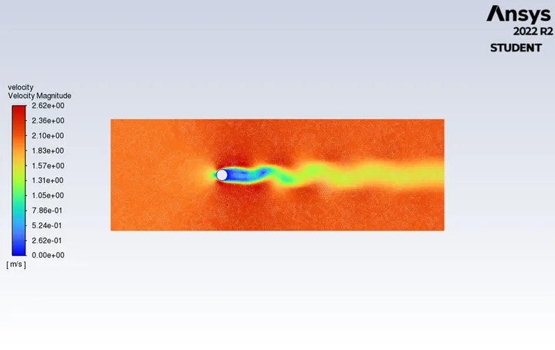
VELOCITY:

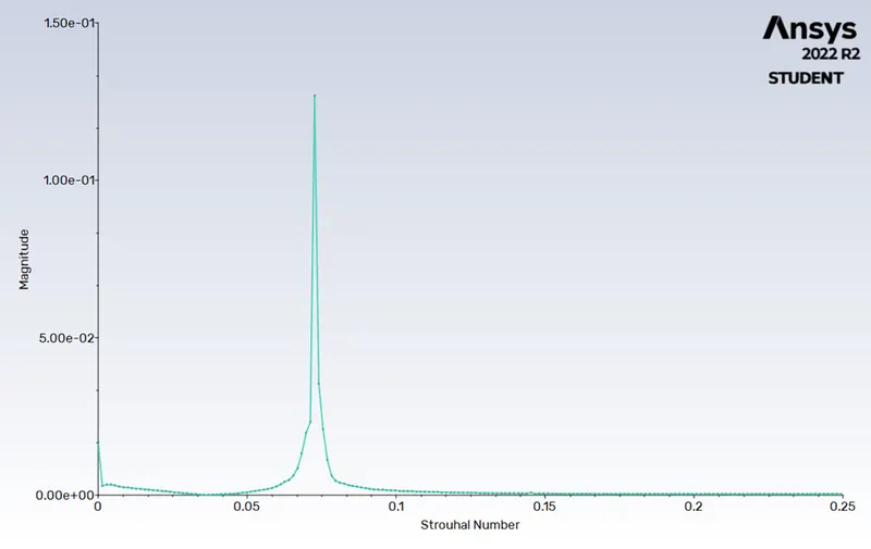
STROUHAL NUMBER:

From above plots and figures observations explained below

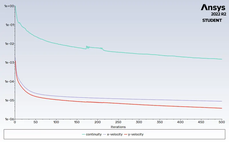
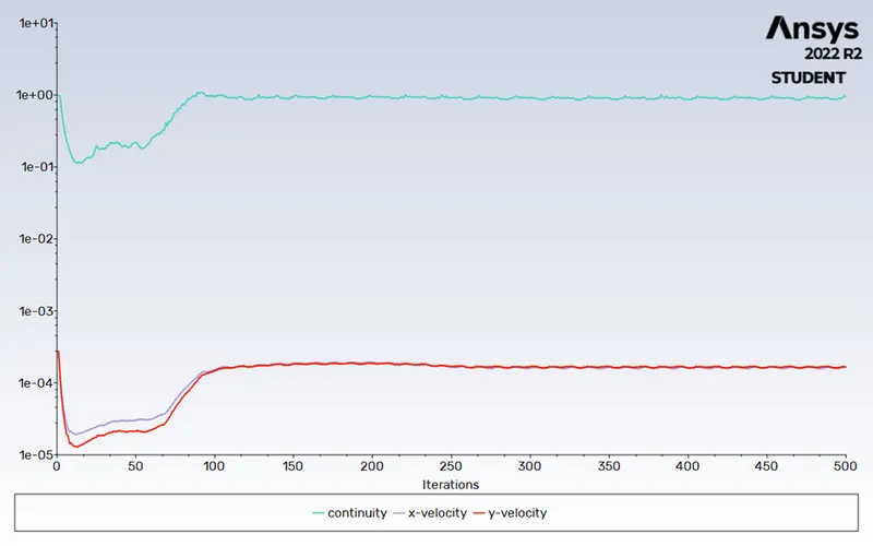
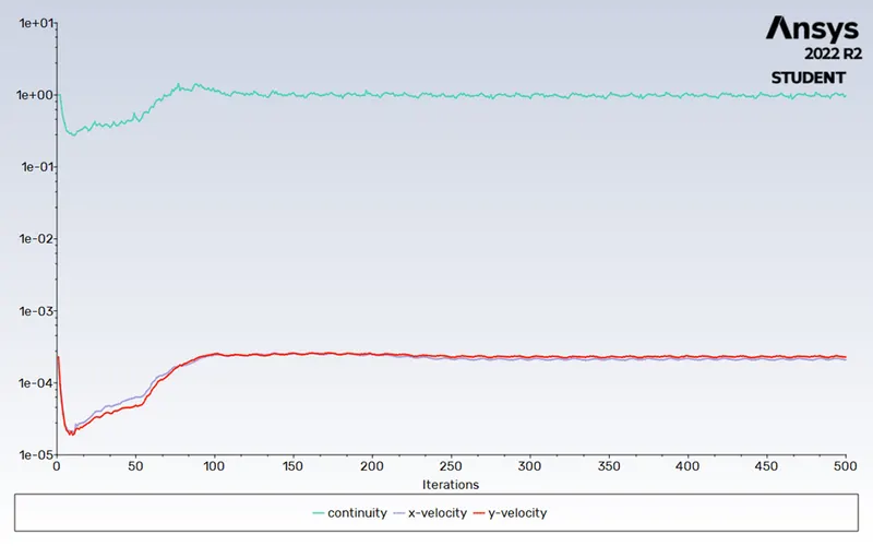
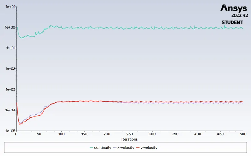
1. In residual plot, the error value is neither changing not increasing from the set limit of 1e-3, that's why it can be said that the solution is converged.
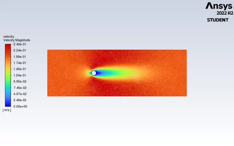
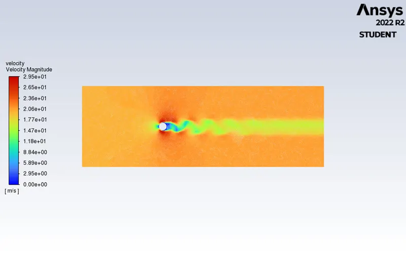
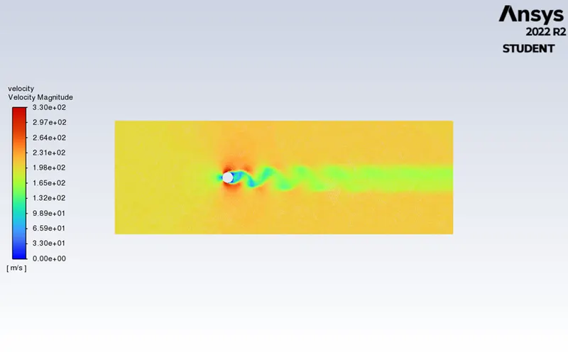
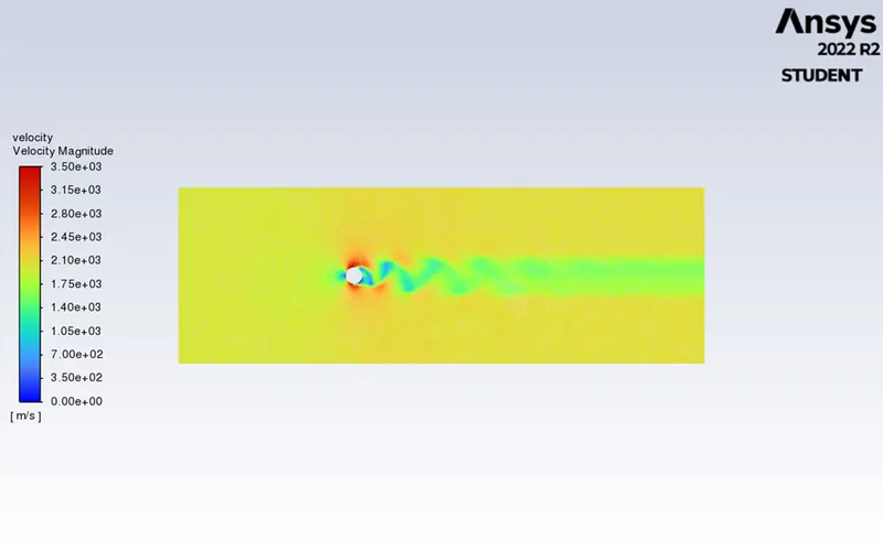
2. In velocity contour plot, the von kamran vortex street is visible in that the flow of velocity flows from cylinder.
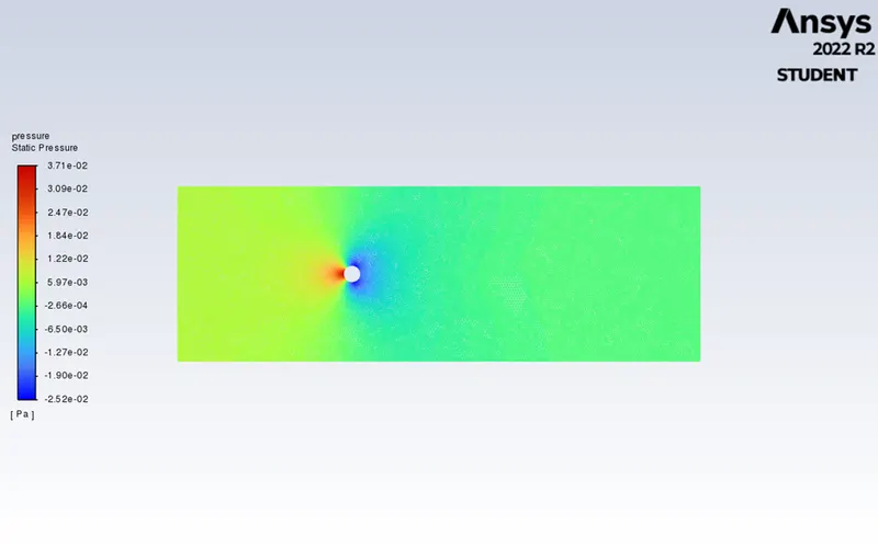
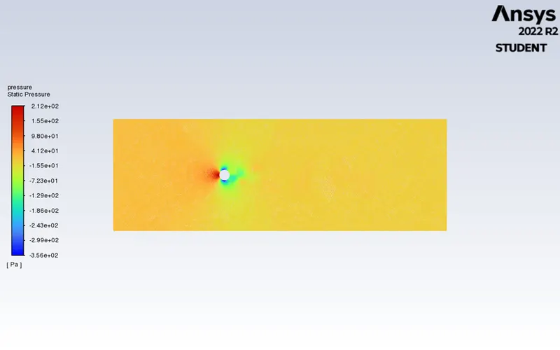
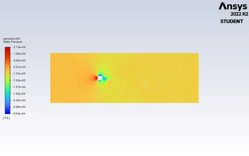
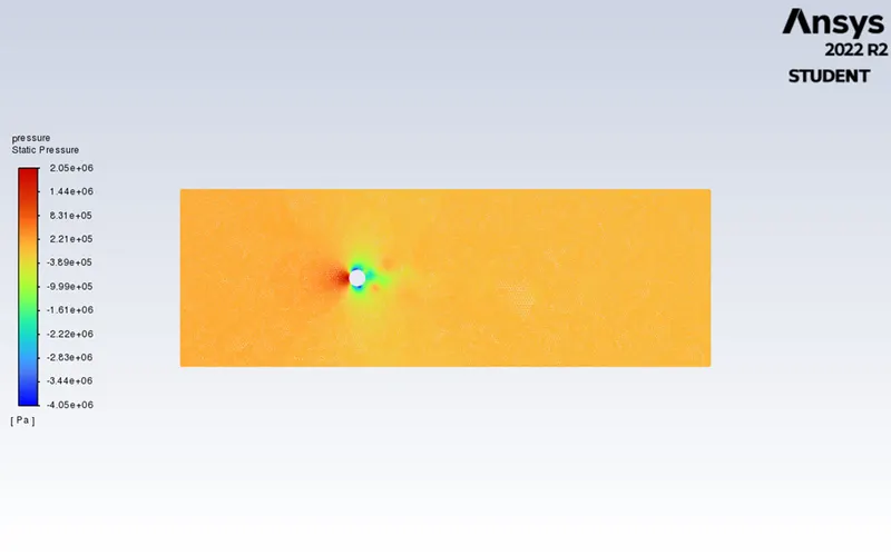
3. In pressure contour image, the low-pressure field is changing alternately. It can be seen by observing the blue area. The low-pressure wake field is the primary physics to observe for this challenge.
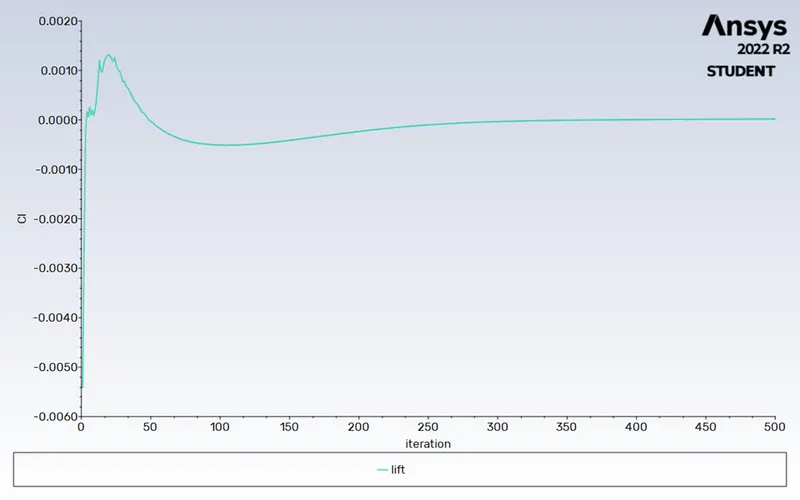
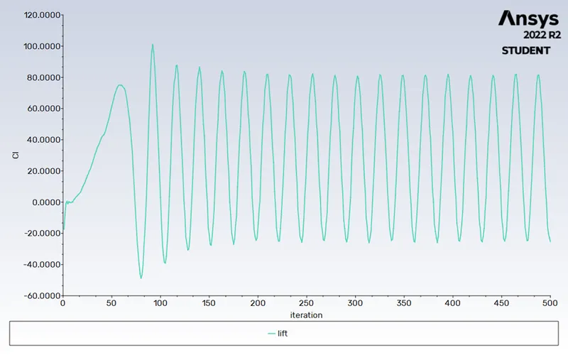
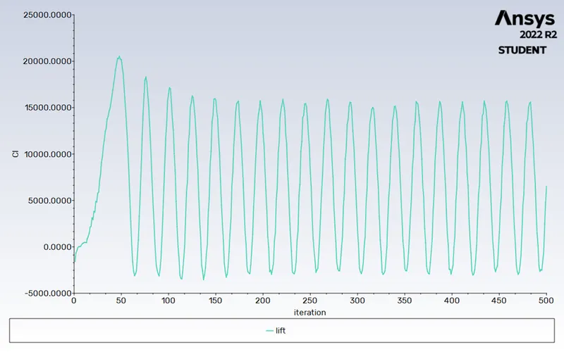
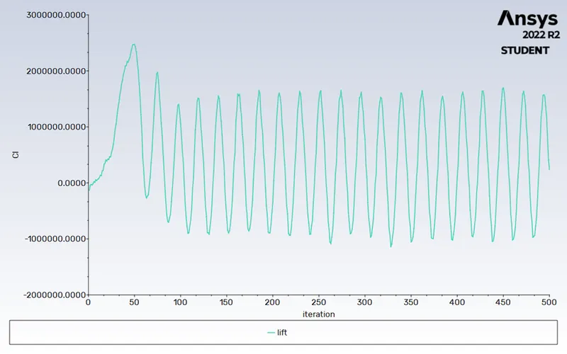
4. In lift coefficient plot, the value is kept rising & falling because of vortex shedding phenomena. The lift coefficient data has been used in the Fourier Transform (FFT) plot to plot the Strouhal number.
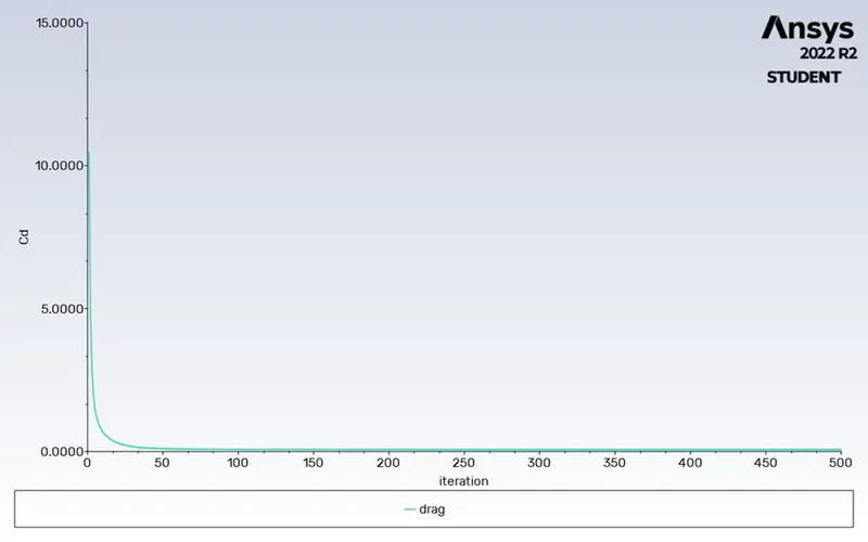
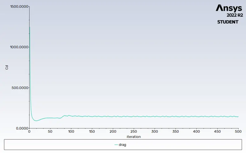
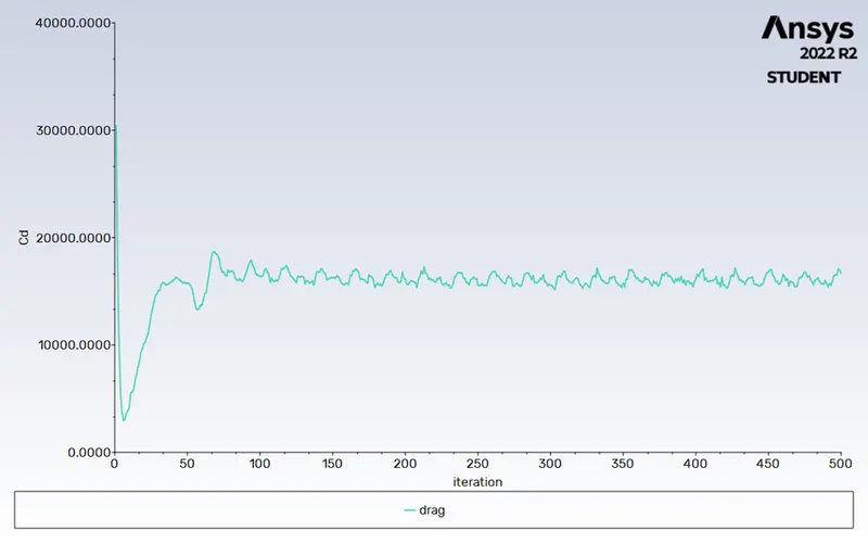
5. The drag coefficient value is constant after one point. The drag coefficient of the cylinder is calculated by the fluent.

The drag coefficient values has been compared with the experimental data provided in the following research paper written by B.N. Rajani which is "Numerical simulation of laminar flow past a circular cylinder". The drag coefficient values are within the 5% variance in comparison with the experimental data.

6. The Strouhal number determined by taking the medium of the plot data in the Fluent software is 0.05 and 0.07 for steady & unsteady state simulation. Through analytical method, the Strouhal number is calculated as 0.16. So, the Strouhal number of fluent is nearer to the analytical method.

CASE 2:

Reynolds Number = Inertial Force / Viscous Force

The Reynolds number formula is expressed by

R_e= ρUL/μ

Where,

ρ = Fluid density

U = Fluid velocity

μ = Fluid viscosity

L = length or diameter of the fluid.

Dynamic Viscosity: 0.04 Kg/m-s

Charecteristics length or diameter: 2 m

Density: 1 Kg/m^3

Reynolds Number	Flow velocity
10	0.2 m/s
100	2 m/s
1000	20 m/s
10000	200 m/s
100000	2000 m/s

For Reynolds Number 10 Results

RESIDUAL:

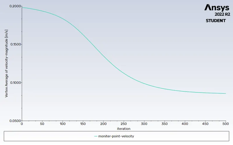
VELOCITY MAGNITUDE:

DRAG COEFFICIENT:

LIFT COEFFICIENT:

PRESSURE:

VELOCITY:

For Reynolds Number 100 result refer case 1 steady state plots and output.

For Reynolds Number 1000 Result

RESIDUAL:

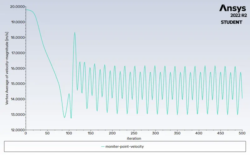
VELOCITY MAGNITUDE:

DRAG COEFFICIENT:

LIFT COEFFICIENT:

PRESSURE:

VELOCITY:

For Reynolds Number 10000 Results

RESIDUAL:

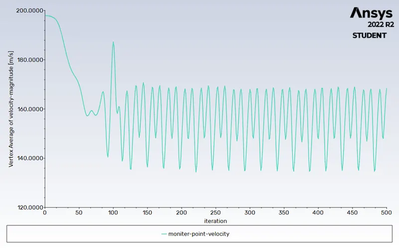
VELOCITY MAGNITUDE:

DRAG COEFFICIENT:

LIFT COEFFICIENT:

VELOCITY:

PRESSURE:

For Reynolds Number 100000 Results

RESIDUAL:

LIFT COEFFINCIENT:

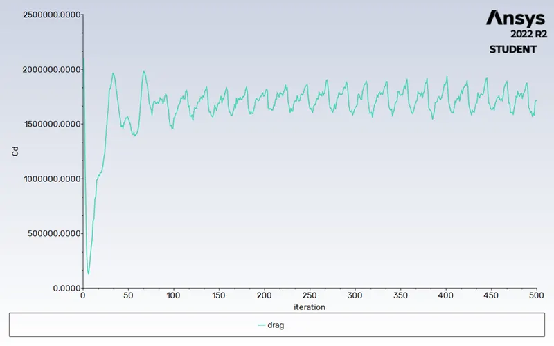
DRAG COEFFICIENT:

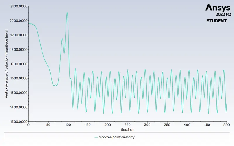
VELOCITY MAGNITUDE:

VELOCITY:

PRESSURE:

RESULTS AND CONCLUSION:

The drag coefficient for the Re above 1000, is start fluctuating but periodic after one point which can be seen from the results images. So statistically, it is constant.

The challenge of simulating flow over a cylinder has been carried out to study the vortex shedding phenomena & visualizing von karman vortex street. The challenge has been divided into two parts. In first part, the steady& unsteady state simulations have been performed for Re 100 & Strouhal number has been calculated using analytical method & later compared with the fluent result. While in second part series of simulation has been carried out for various Re numbers in steady state position. Vortex shedding & karman vortex street was unable to visualize for Re 10 because these two phenomena doesn’t occur below Re 40. The drag coefficient & lift coefficient has been compared for all simulations.

The time & resources consumes by the transient solver is far more than the steady state solver.

For the transient simulations, the simulation were running after turning off the convergence criteria. In transient mode, the more iterations are required to develop proper physics of the flow. Because of that the transient simulation has taken more iteration with smaller time steps compare to the steady state.

REFERENCES:

CFD Modeling of Flow Over a Cylinder · CFD Flow Engineering

Laminar Flow Over a Cylinder: Study1 #1 (nasa.gov)

https://en.wikipedia.org/wiki/K%C3%A1rm%C3%A1n_vortex_street