Week 2 - Flow over a Cylinder.

AIM:

Simulate the flow over a 2D cylinder and explain the phenomenon of Von Karman vortex street. Here the diameter of 2D Cylinder is set to 2m.

PART-I

1. Simulate the flow with the steady and unsteady case and calculate the Strouhal Number for Re= 100.

PART-II

1. Calculate the coefficient of drag and lift over a cylinder by setting the Reynolds number to 10,100,1000,10000 & 100000. (Run with steady solver)
2. Discuss the effect of Reynolds number on the coefficient of drag. [ Results should be validated with any standard literature and error should be within 5 %]

OBJECTIVE:

1. To check the convergence of flow.
2. Plots of coefficients of drag and lift.
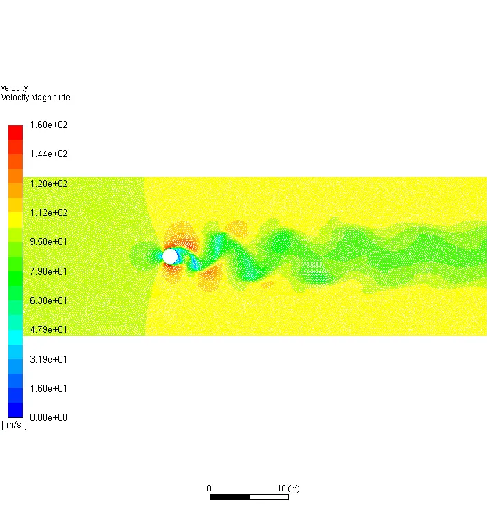
3. Plots to show vortex shedding behind the cylinder.
4. Discuss the effect of length and momentum ratio on results.

INTRODUCTION:

This simulation is intended to understand the variation of flow regimes when fluid flows over a 2D cylinder. Here the body wall surface of cylinder is stationary which indeed creates a no-slip condition and hence a boundary layer is formed around the wall. But it should be noted that as free stream velocity increases the velocity gradient normal to wall surface increases which subsequently gives rise to boundary layer separation. The increase in velocity is characterised by Reynold’s number. It should be also noted that the very sharp velocity gradient near the wall surface makes it so non-linear profile that it becomes difficult for the CFD solver to predict the flow near the surface. So, from studies and literatures it was found that there exists a dimensionless number named y+ which indeed helps in predicting first mesh centroid length from wall. This y+ value when less than 1 we get approximate better values for first centroid distance from wall. When free stream velocity increases Reynold’s number increases which there by increases the turbulence characteristics of the flow field. Turbulence with boundary layer separation along the circumference of the circular cross-section of cylinder there by forms shear layers along the symmetry of the circular cross-section which flows at different velocities. These different velocity shear layers moving tangentially to the circle will create a vortex shedding. This phenomenon is known as Von Karman Vortex Street. This oscillating flow is quantified by a dimensionless number named Strouhal number. Finally due to variation in velocity and pressure there would be formation of lift and drag. These changes in lift and drag and accounted by coefficient of drag and lift.

THEORY:

Reynold’s number:

Reynolds number is the ratio of inertia force to viscous force.

Where,

Y+ Calculation :

Y+ = (V_f x Y_p)/V_w

Where V_f is friction velocity and Y_p is distance from wall to first cell centroid and V_w is kinematic viscosity at wall.

V_f= sqrt(T_w/ )

Where T_w= Shear stress at wall

And is density

T_w= 0.5 x C_d x x A x V²

Where C_d is coefficient of drag and A is frontal area and V is free stream velocity

And C_d= 0.0576 x Re^0.2

Assume Re is 100, then C_d=0.0145

If is 1 and Area of cross-section is 3.14 and V is 1 then T_w is 0.0228.

Now V_f is 0.15.

Now let Y+ be 0.5 and V_w is 0.02 then Y_p will be 0.067 m. Here we will be choosing some value less than 0.005 m since Re 10 is also needed to be evaluated.

Strouhal Number:

Strouhal number is a dimensionless number which describes and quantitavelu measure the oscillating mechanisms.

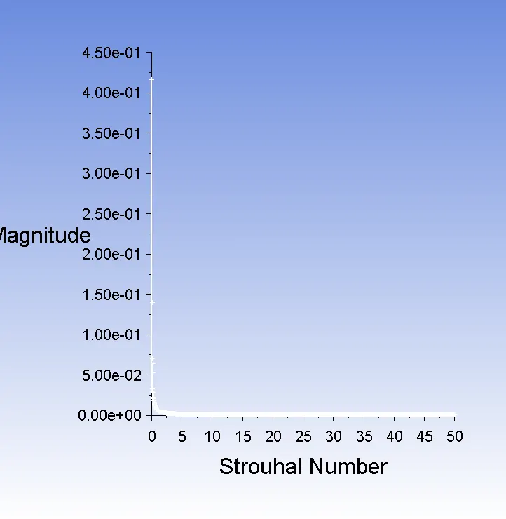
St= (Fst x D)/V where Fst is the vortex shedding frequency, D is the diameter of circular cylinder and V is free stream Velocity.Y axis as magnitude and X axis as Strouhal number.

PROCEDURE:

PART:1

SOLVING AND MODELLING APPROACH:

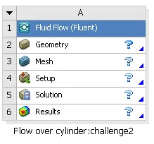
1. Re= 100, D = 2m, V=1m/s, is 1 kg/m³, the V_w= 0.02 Ns/m².
2. Computational Domain:

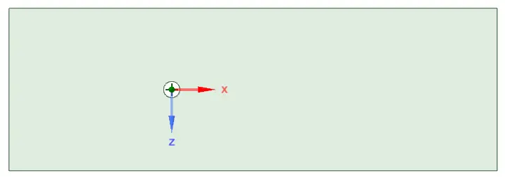
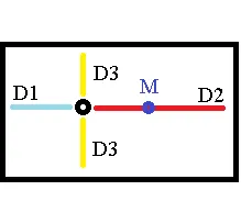
Diameter of Circle= 2m

D1= Frontal Distance = 10D= 20m

D2= Rear-Side Distance=20D= 40m

D3= 5D= 10m

M is the location of monitor point chosen for measuring the variation in oscillation and velocity in the wake side of cylinder

PREPROCESSING AND SOLVER SETTING:

MESH SETTING:

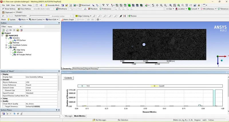
1. Triangular-Tetrahedral Mesh pattern is selected.
2. Element size is set to 0.25
3. 10 inflation layers with base layer mesh height set to 0.005m and growth rate of 1.2 is given around the cylinder

SOLVER SETTING (Steady State):

1. Model: Pressure based – Steady state flow, Viscous -Laminar condition selected.
2. Materials= User defined air with kinematic viscosity 0.02 NS/m² and Density = 1kg/m³.
3. Boundary Conditions:
   100. Inlet- velocity with magnitude 1m/s to make Reynold’s number 100.
   101. Outlet- Pressure based- Gauge pressure 0
   102. Cylinder wall- No slip condition and stationary boundary.
   103. Symetric wall- Symmetry Boundary Condition.

4. Reference values – Length 2m and A= 2m changed. Remaining all same.
5. Method: SIMPLE Algorithm with default wall conditions.
6. Convergence criteria turned off to get Entire flowfield.
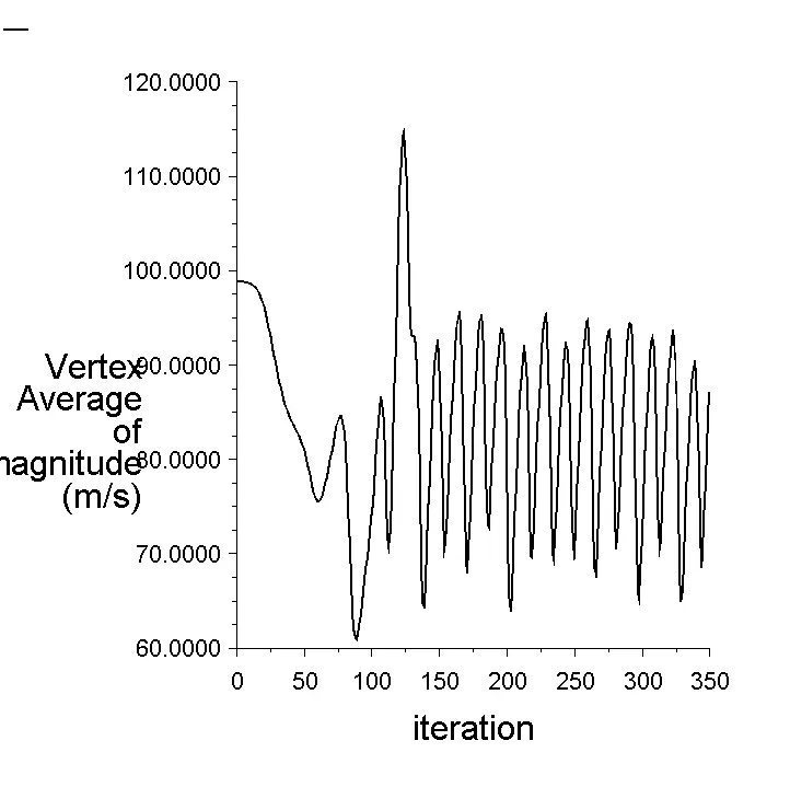
7. Defined monitor point from Post processing and in Solving added new definition with average vertex velocity value at the defined monitor point.
8. Selected Hybrid Initialization and Initialized for 10 iterations.
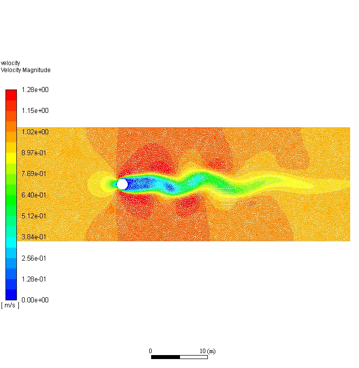
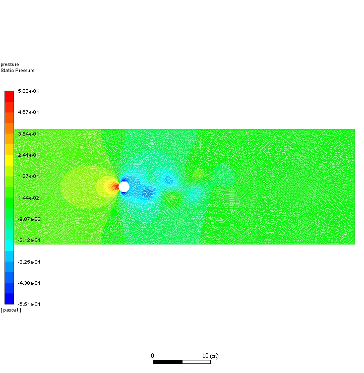
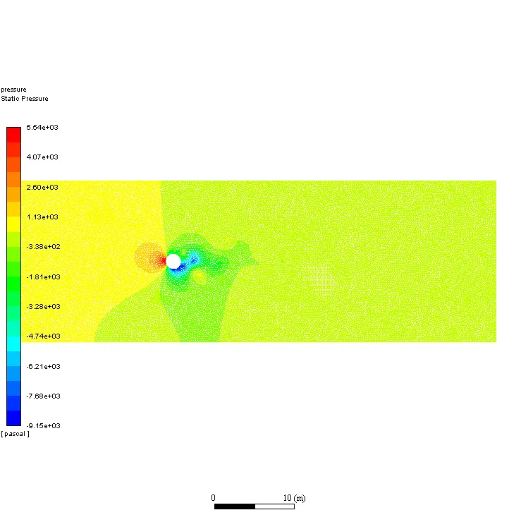
9. Defined new contour plots for velocity and pressure and created animated video foe velocity contour.
10. Set 350 iterations and run calculations.

SOLVER SETTING (Transient State):

1. Model: Pressure based – Transient state flow, Viscous -Laminar condition selected.
2. Materials= User defined air with kinematic viscosity 0.02 NS/m² and Density = 1kg/m³.
3. Boundary Conditions:
   100. Inlet- velocity with magnitude 1m/s to make Reynold’s number 100.
   101. Outlet- Pressure based- Gauge pressure 0
   102. Cylinder wall- No slip condition and stationary boundary.
   103. Symetric wall- Symmetry Boundary Condition.

4. Reference values – Length 2m and A= 2m changed. Remaining all same.
5. Method: SIMPLE Algorithm with default wall conditions.
6. Convergence criteria set to 0.0000001 to get Entire flow field.
7. Defined monitor point from Post processing and in Solving added new definition with average vertex velocity value at the defined monitor point.
8. Selected Standard Initialization and defined time step of 0.01 for 4700 number of steps. i.e91720 iterations.
9. Defined new contour plots for velocity and pressure and created animated video foe velocity contour.
10. Run Calculations.
11. FFT with X-axis Strouhal number and Y-axis Magnitude is plotted to calculate Strouhal number.

PART:2

SOLVING AND MODELLING APPROACH:

3. Re= 10, D = 2m, V=0.1m/s, is 1 kg/m³, the V_w= 0.02 Ns/m².
4. Computational Domain:

Diameter of Circle= 2m

D1= Frontal Distance = 10D= 20m

D2= Rear-Side Distance=20D= 40m

D3= 5D= 10m

M is the location of monitor point chosen for measuring the variation in oscillation and velocity in the wake side of cylinder

PREPROCESSING AND SOLVER SETTING:

MESH SETTING:

4. Triangular-Tetrahedral Mesh pattern is selected.
5. Element size is set to 0.25
6. 10 inflation layers with base layer mesh height set to 0.005m and growth rate of 1.2 is given around the cylinder

SOLVER SETTING (Steady State):

11. Model: Pressure based – Steady state flow, Viscous -Laminar condition selected.
12. Materials= User defined air with kinematic viscosity 0.02 NS/m² and Density = 1kg/m³.
13. Boundary Conditions:
    100. Inlet- velocity with magnitude 1m/s to make Reynold’s number 100.
    101. Outlet- Pressure based- Gauge pressure 0
    102. Cylinder wall- No slip condition and stationary boundary.
    103. Symetric wall- Symmetry Boundary Condition.

14. Reference values – Length 2m and A= 2m changed. Remaining all same.
15. Method: SIMPLE Algorithm with default wall conditions.
16. Convergence criteria turned off to get Entire flowfield.
17. Defined monitor point from Post processing and in Solving added new definition with average vertex velocity value at the defined monitor point.
18. Selected Hybrid Initialization and Initialized for 10 iterations.
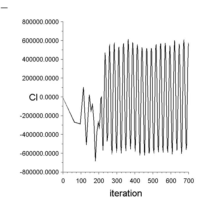
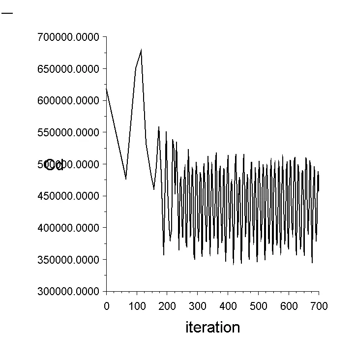
19. Defined new contour plots for velocity and pressure and created animated video foe velocity contour and defined new plots for lift and drag coefficients.
20. Set 350 iterations and run calculations.

Here Re was 10, D = 2m, V=0.1m/s, is 1 kg/m³, the V_w= 0.02 Ns/m².(Repeat the above same steps for Re 100,1000,10000,100000 by changing Velocity to 1m/s, 10m/s,100m/s and 1000m/s respectively.

RESULT:

PART:1

STEADY STATE Re=100

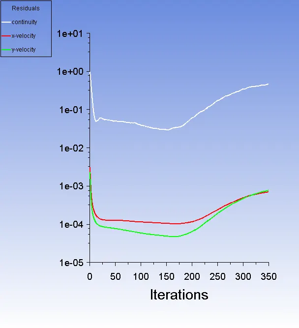
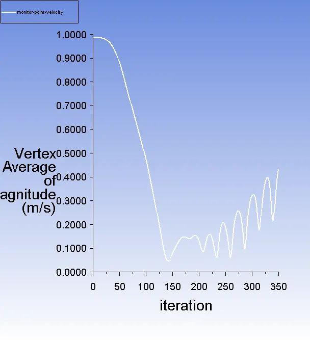
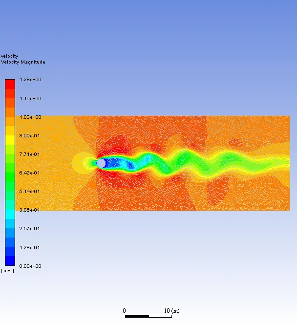
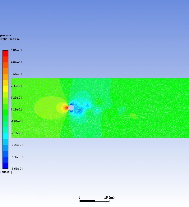
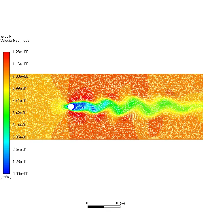
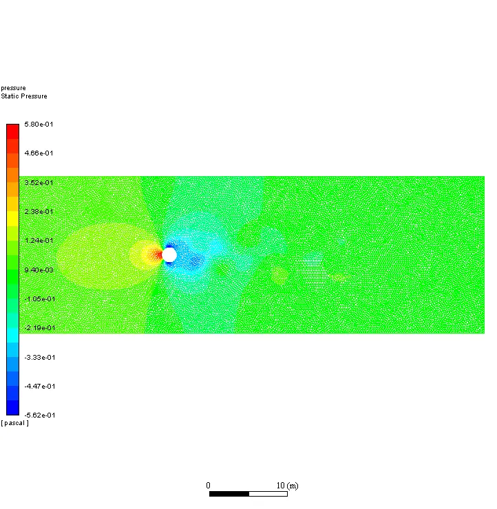
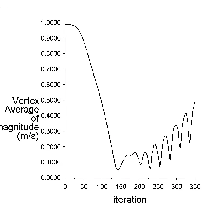
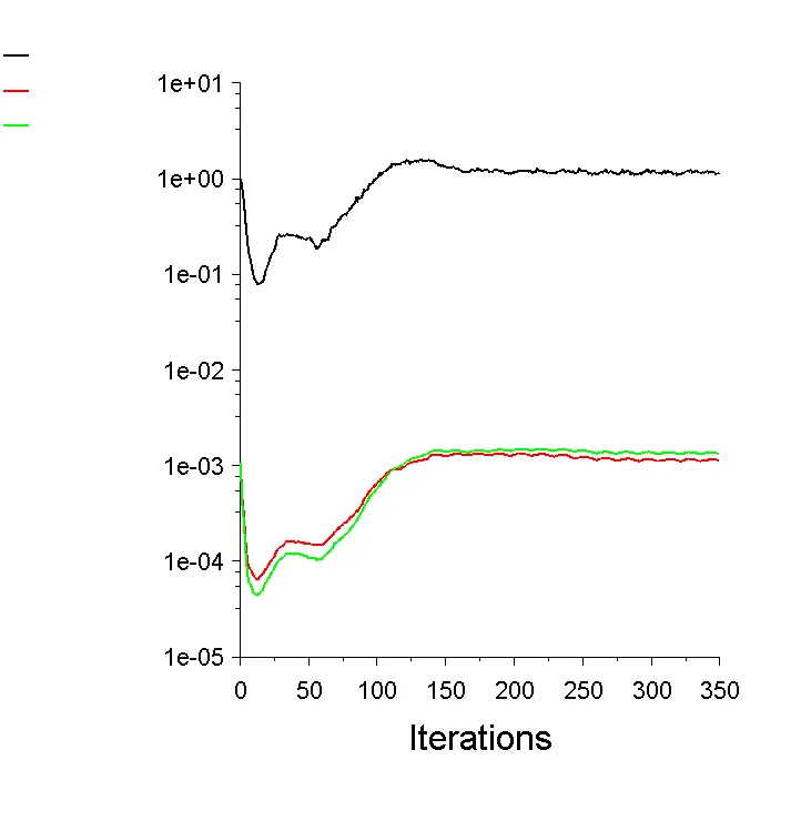
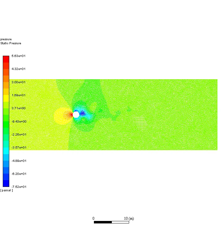
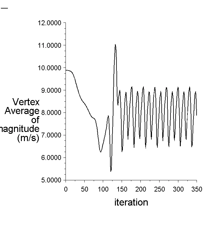
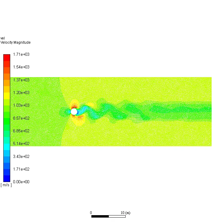
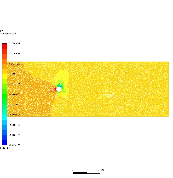
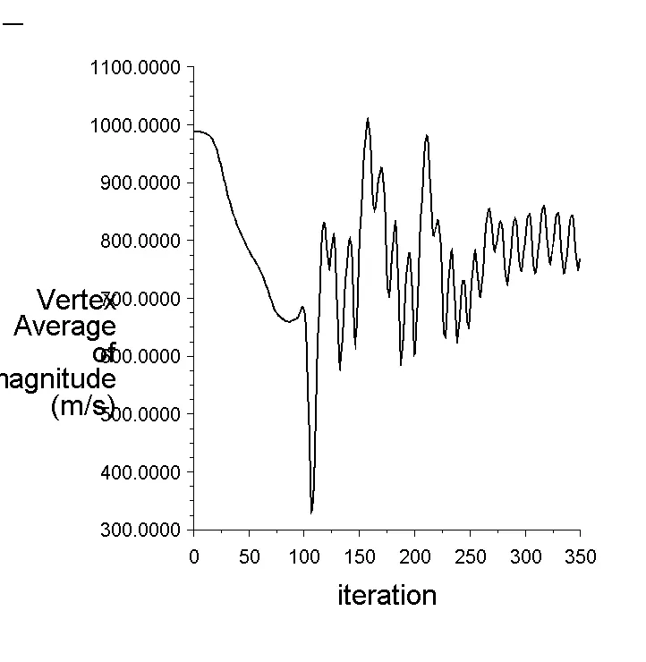
1. Steady state convergence, average velocity at monitor point and velocity, pressure contour plots are made.

TRANSIENT STATE Re=100

1. Transient state convergence(Residuals), average velocity at monitor point and velocity, pressure contour plots are made and FFT with X-axis Strouhal number and Y-axis Magnitude is plotted.

   PART:2

   STEADY STATE

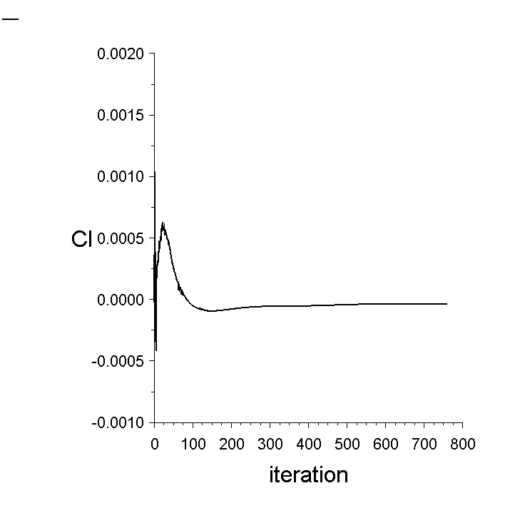
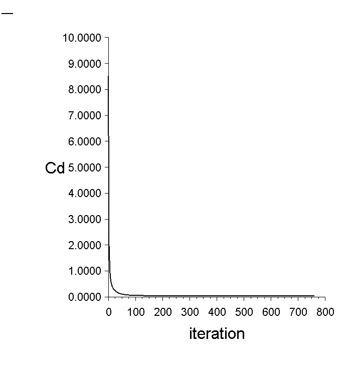
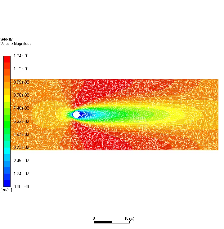
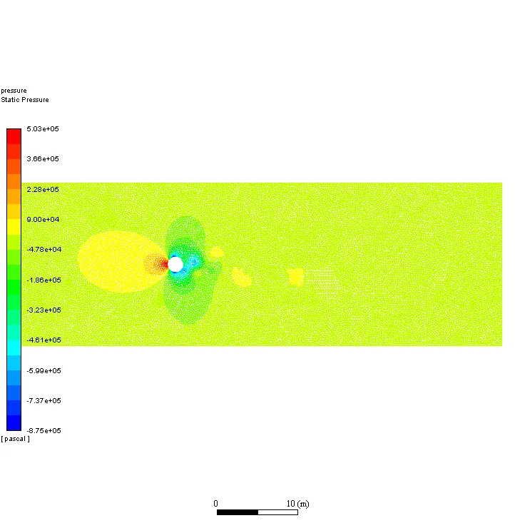
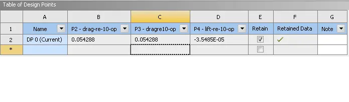
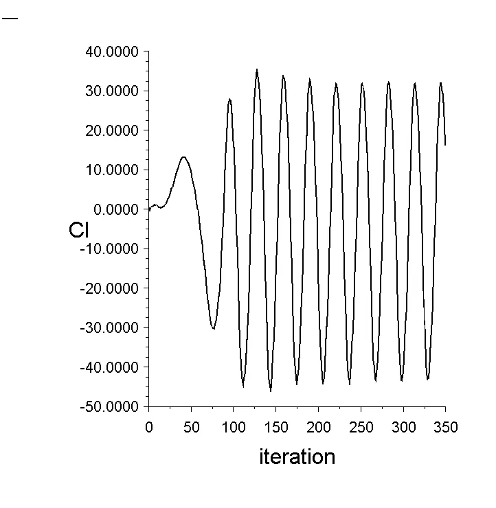
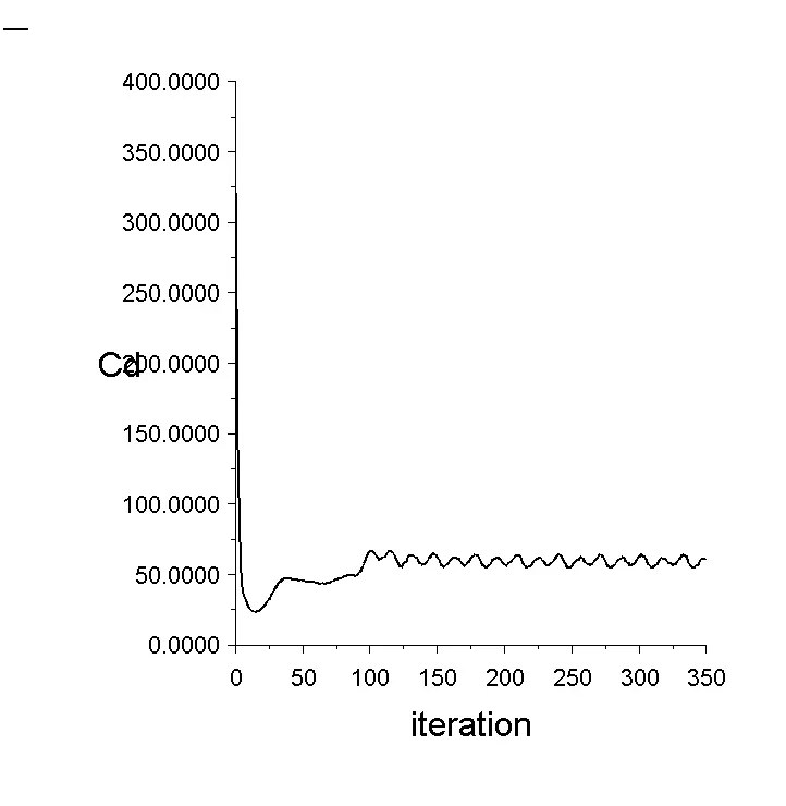
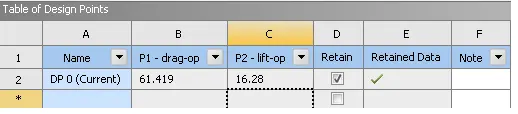
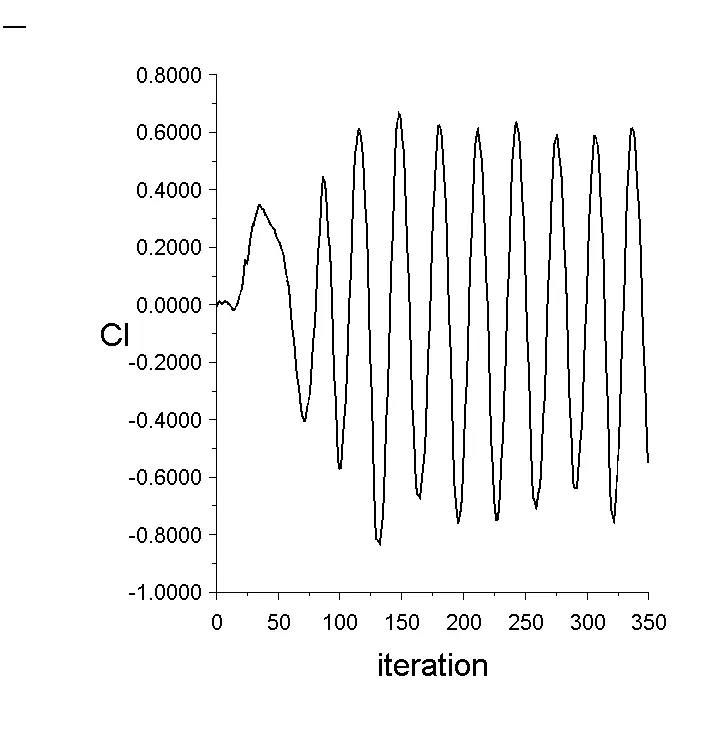
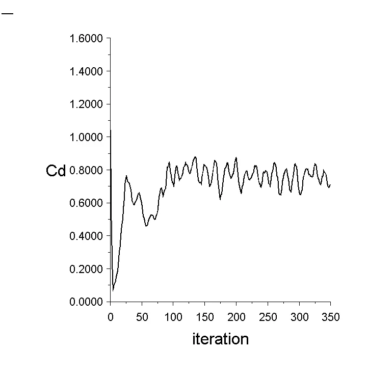
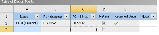
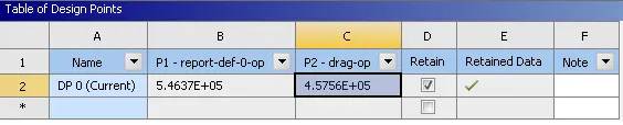
   At different Reynold’s number obtained from different velocities the variation in coefficient of drag and lift was observed.

   1.Re:10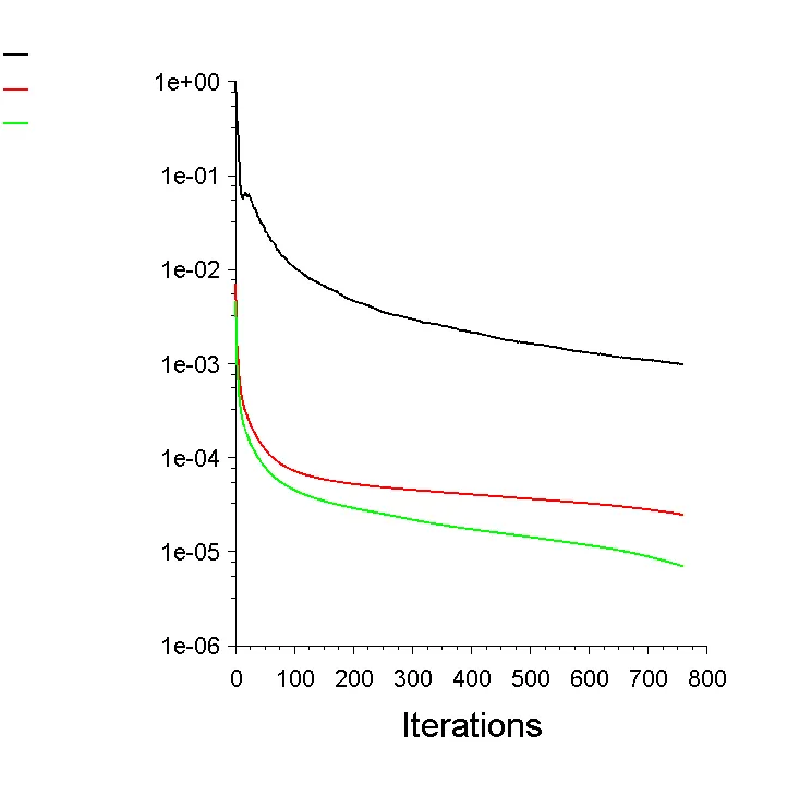2. Re=100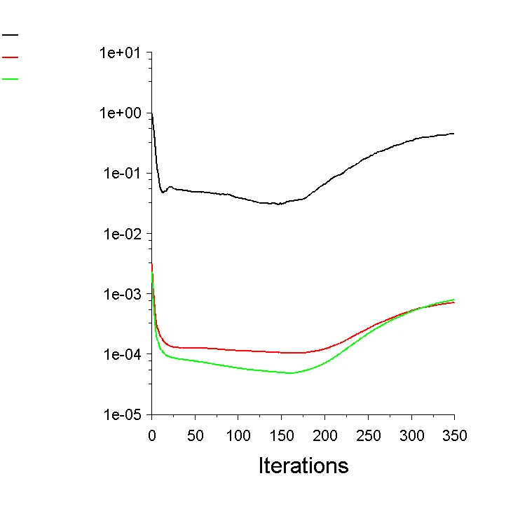
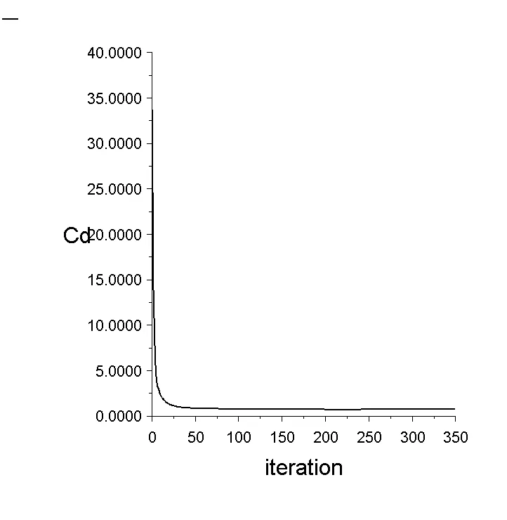
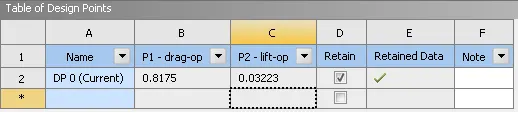
2. Re:10004.Re:10000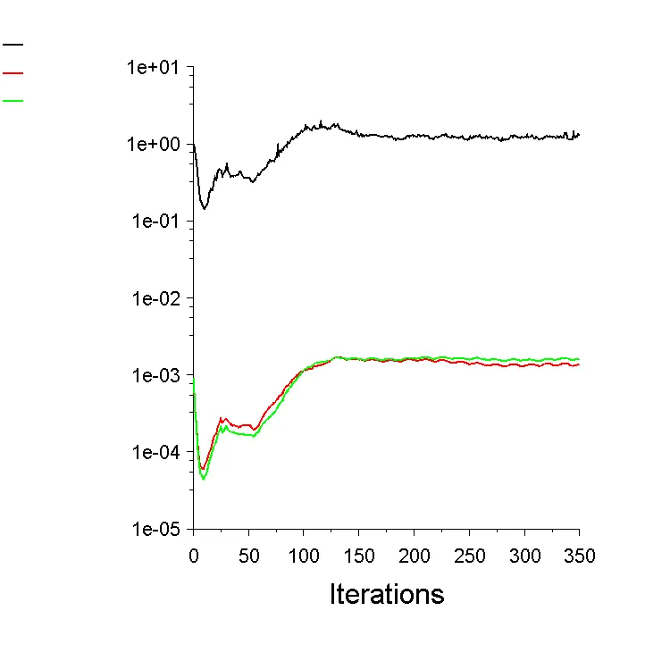5. Re:100000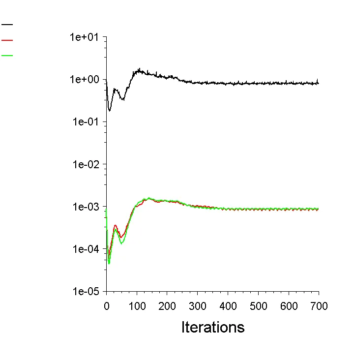

CONCLUSION:

PART:1

STEADY STATE Re=100

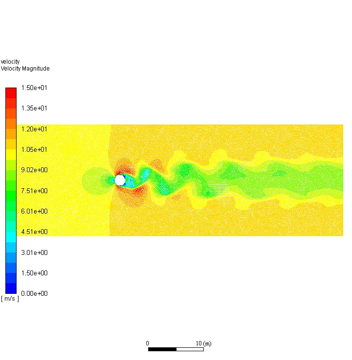
1. It was observed to show Vortex shedding as mentioned in literatures after 165^th iterations and vertex velocity at monitor point started oscillating with increasing amplitude. Now to capture Vortex shedding and calculate Strouhal number we need to go for transient(unsteady)approach.

TRANSIENT STATE Re=100

1. Vortex shedding was observed with more clarity and Strouhal number plot was made. animation link of velocity contour https://drive.google.com/file/d/1_U4JZJNrIiw1B2sj_qGeIDlOF2PLhx8M/view?usp=sharing

PART:2

STEADY STATE

At different Reynold’s number obtained from different velocities the variation in coefficient of drag and lift was observed.

REFERENCES:

1. Anderson J.D,”Fundamentals of Aerodynamics”, 2^nd Ed,Ch.3:pp.229
2. Shames I.H,”Mechanics of fluid”, 3^rd, Ch.13:pp.669-675