Week 2 - Flow over a Cylinder.
Aim- Simulate the flow over a cylinder
theory-
The Strouhal Number is a dimensionless value useful for analyzing oscillating unsteady fluid flow dynamics problems.
The Strouhal Number can be expressed as
St = ω l / v
where
St = Strouhal Number
ω = oscillation frequency
l = characteristic length
v = flow velocity
Von Karman Street:-
In fluid dynamics, a Von Karman Street is a repeating pattern of swirling vortices, caused by a process known as vortex shedding, which is responsible for the unsteady separation of flow of a fluid around blunt bodies.
Inflation layer-
fine layerss of cell, it is used to capture the simulation accurately for a certain region it is a set of thin layers that keep on in increasing in size as we move outwards.
Boundary layers-
boundary layer, in fluid mechanics, thin layer of a flowing gas or liquid in contact with a surface such as that of an airplane wing or of the inside of a pipe. The fluid in the boundary layer is subjected to shearing forces. A range of velocities exists across the boundary layer from maximum to zero, provided the fluid is in contact with the surface. Boundary layers are thinner at the leading edge of an aircraft wing and thicker toward the trailing edge. The flow in such boundary layers is generally laminar at the leading or upstream portion and turbulent in the trailing or downstream portion
Procedure-
1) first we need to ope space claim and create our geometry
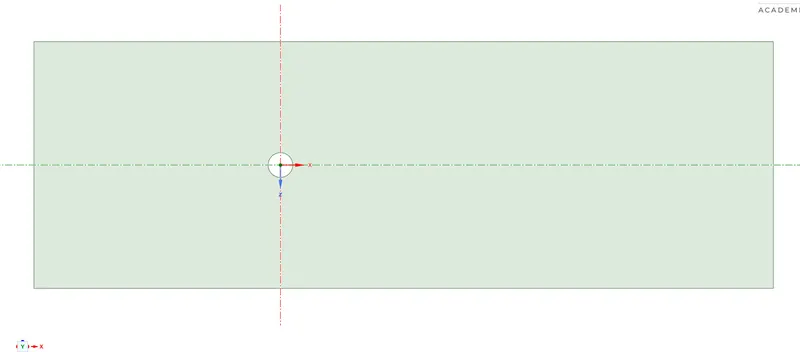
2)open space clain go to sketch mode here we can draw a cylinder and a plane and as we exit out of sketch mode to 3d mode it will be automatically converted to a plane(our dia is 2m and retangle 60 m x 20m)
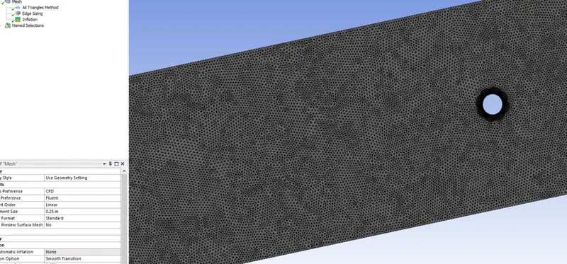
3) now that we have created geometry me can continue to meshing, to want to preserve shape of the cylinder we will use trias instead of quad geometry we can do that by adding a method to mesh
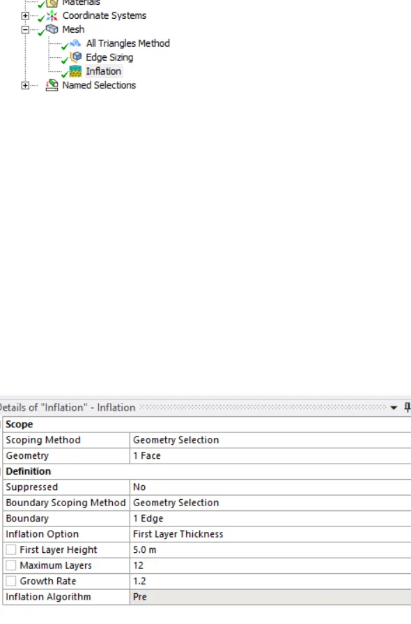
4)similarly we will also add infaltion layers and edge sizing(200 division) we are using inflation layers to properly capture boundary layers(12 layers growth rate 1.2 max layers 12)
5)now using shortcut key n we can use name edges i.e inlet outlet and cylinder wall
6)now we can move to setup deck where we can set config to-
general- solver -pressure based, time - steady
Models- Viscous model:- Laminar
materials- copy air properties density - 1000kg/m3 viscosity =.02
inlet vel= velocity is varied to for diff cases to change reynols no using (re=rho *V*D/nu)
solution method= simple
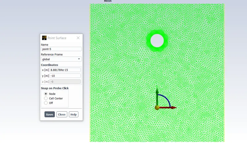
8) create a monitor point 8m away from centre of cylinder by results>>surface>create
9) create reports for lift and drag and one for the monitor point.
10) now we have to enter the ref value only velocity and viscosity needs to be changes acqdingly
11) now we can initialize and create a solution animation after we can run for 200 iteration
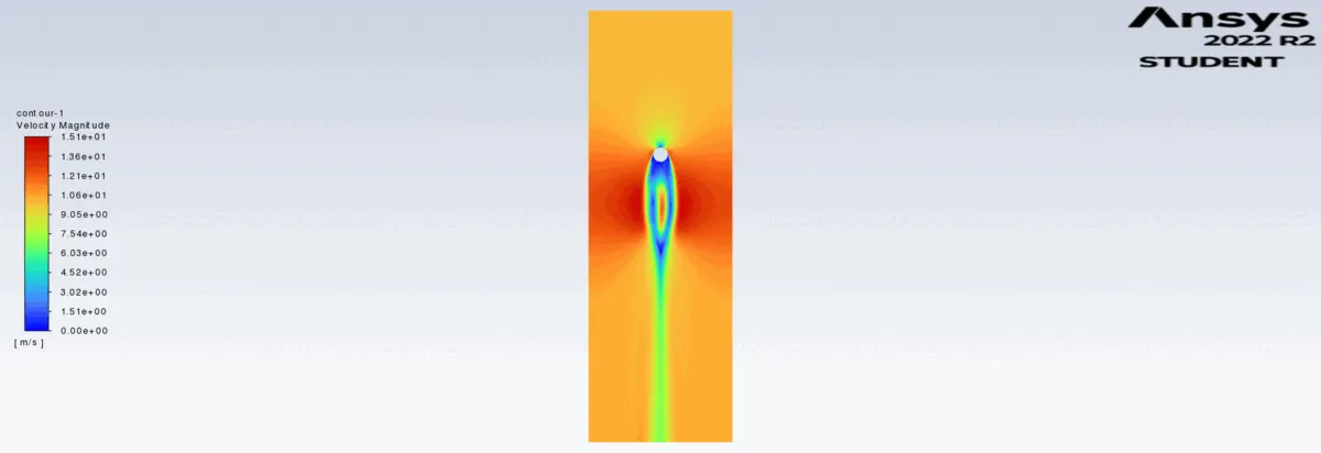
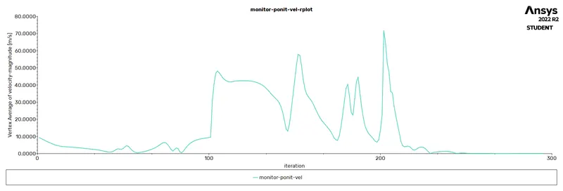
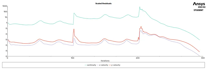
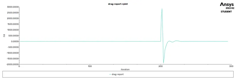
results re=100
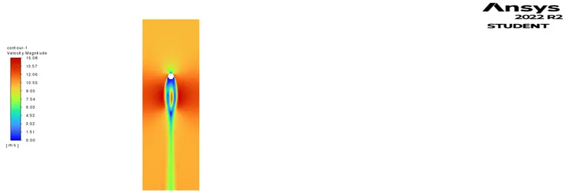
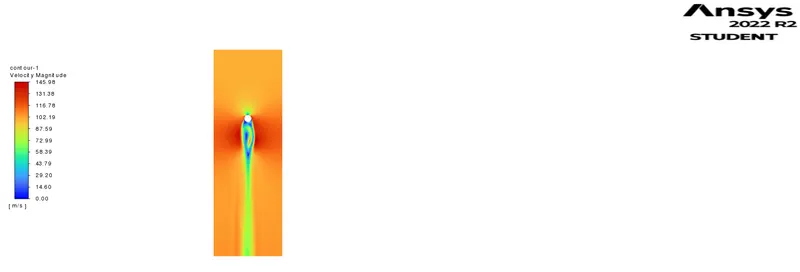
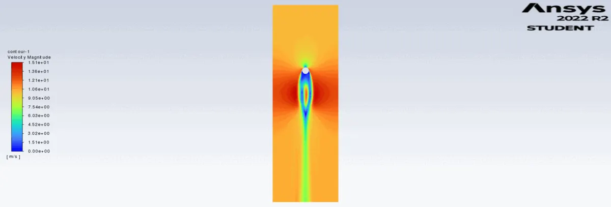
vel contour-
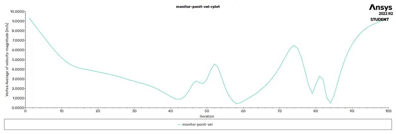
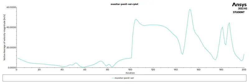
vel at monitor point-
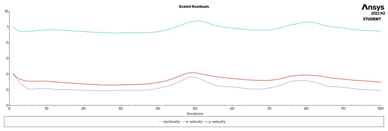
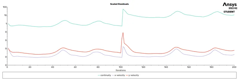
residual plot-
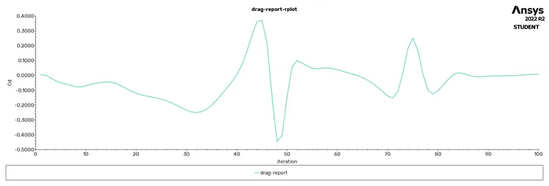
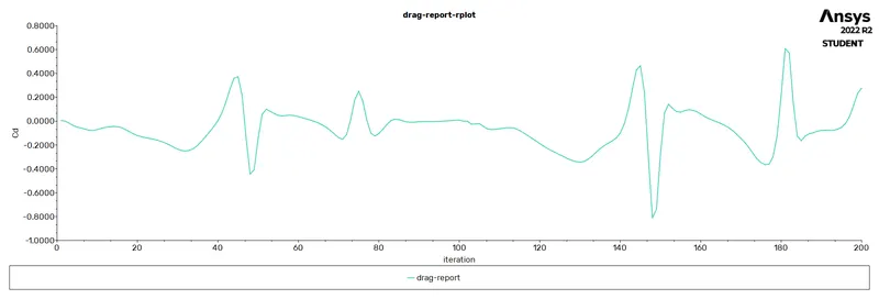
drag plot-
Plots for re = 1000-
drag plot-
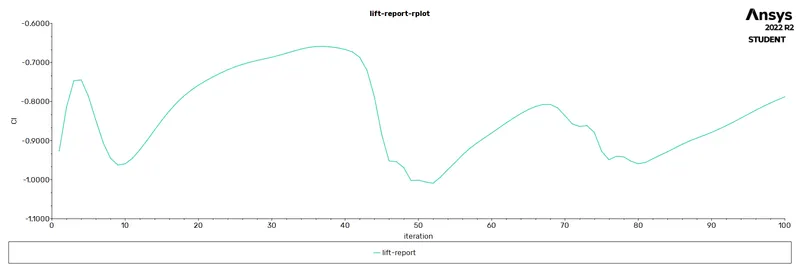
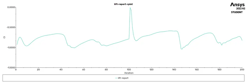
lift plot-
monitor point-
residual plot-
velocity graph-
plots for re 10000-
drag plot -
lift plot-
monitor point-
residual plot-
velocity plot
vel plot for re=100 and viscosity is increased to .05-
conclusion- as we can see as the reynols no increases drag decrease