Week 2 - Flow over a Cylinder.
`
Abstract
The present work focuses on the analysis of two-dimensional flow past a circular cylinder and determining the variation in the coefficient of lift and drag over the cylinder at Reynolds number 10,100,1000,10000,100000. In addition to this, the Strouhal Number is calculated to describe the oscillating flow mechanism past the cylinder.
Two-Dimensional Flow over the Cylinder
Introduction
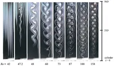
The generation of vortices depends upon the Reynolds number. At lower values of Reynolds number (Re<0.5), inertia forces are negligible as compared to the viscous forces and the drag is proportional to the velocity V. With an increase in the Reynolds number, the flow pattern becomes asymmetrical about the axis perpendicular to the direction of the flow. At Reynolds number ranging from about 2 to 30, very weak vortices are formed the downstream of the cylinder. It is the initial stage for the development of the wake. In the wake region there exist a flow in the opposite direction along the axis of the wake. At Re ranging from about 40 to 70, the wake, as well as the pair of vortices, become quite distinct. With a further increase in the value of Reynolds number the vortices become more and more elongated in the direction of flow, and at Re equal to about 90 these vortices become symmetrical and slowly move in the downstream direction. This work relates the study of wake mechanisms over the cylinder by using ANSYS FLUENT software.
Karman Vortex Trail:
When the Reynolds number exceeds about 30, the two vortices behind the cylinder get stretched and become unstable and are washed down. At the place of washed two vortices two new vortices are created and the process continues. Under such circumstances, the wake behind the cylinder consists of a series of vortex pairs moving in the downstream direction with relatively small velocity. This phenomenon is called Karman Vortex Trail.
Strouhal Number:
Strouhal number represents the ratio of inertial forces due to the local acceleration of the flow to the inertial force due to convective acceleration. At higher Strouhal number oscillation dominates fluid flow. At lower Strouhal number oscillations are washed away by the fluid flow. When the frequency of the lateral force is equal to the natural frequency of the cylinder, resonance will be generated and the lateral force of large magnitude will be generated. Such consideration is very much important in the aerodynamic study of suspension bridges.
The frequency of the lateral force is given by the empirical formula

Geometry
Model
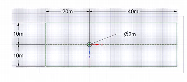
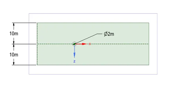
The model is created by using space claim in ANSYS fluent. At first, circle is drawn with the diameter =2m. Then an enclosure i.e. rectangle of 20*60 m is drawn. Pull command is used to create the surface. After creating the surface by using the Delete button the cylindrical surface is deleted.
Named Selection:
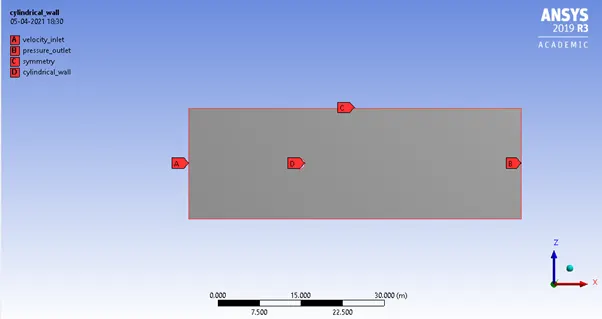
A represents the Velocity inlet through which the fluid enters. B is the outlet for the fluid. C represents symmetrical surfaces. Symmetrical surfaces are used when a large number of similar components are to be analysed. Symmetry reduces computation time. D represents the wall which acts as a barrier for the fluid flow.
Meshing
Meshing is done by using ANSYS software. Element size is chosen to be 0.5m
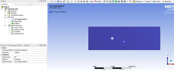
By right-clicking the Mesh option  to generate Triangular Mesh. The triangular mesh will be suitable for complex geometries.
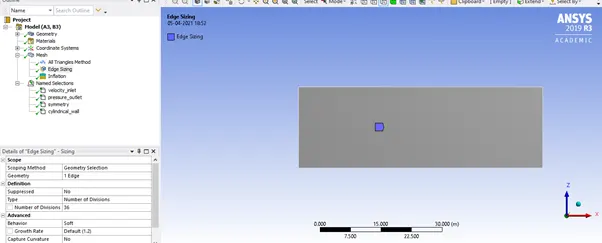
The element size of the wall is controlled by using the Sizing command
 In the sizing option Number of division, the option is selected under the Type option. 36 division is provided to generate finer mesh on the wall.
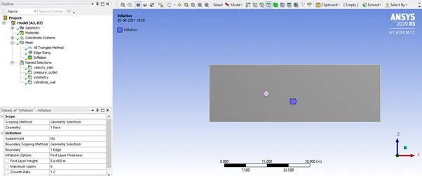
Inflation is used to stack elements/cell in the direction normal to the boundary. Physics at the boundaries are captured effectively when the inflation option is used.
 Under inflation option, the First layer thickness value 5e-3 is used. The maximum layer is 6 is used with the growth rate of 1.2.
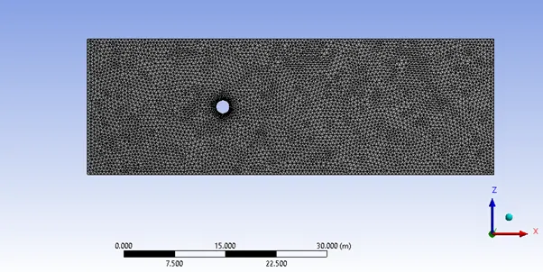
After defining the Mesh details. Generate Mesh is used to develop elements on the surface. Update mesh is used to update the new mesh.
Preprocessing
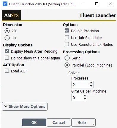
Single precision means that the floating-point numbers will be represented in the 32-bit system whereas double-precision means that they will be represented in a 64-bit system. So calculation in double precision will be more accurate.
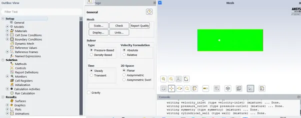
Under Models Viscous laminar is provided.
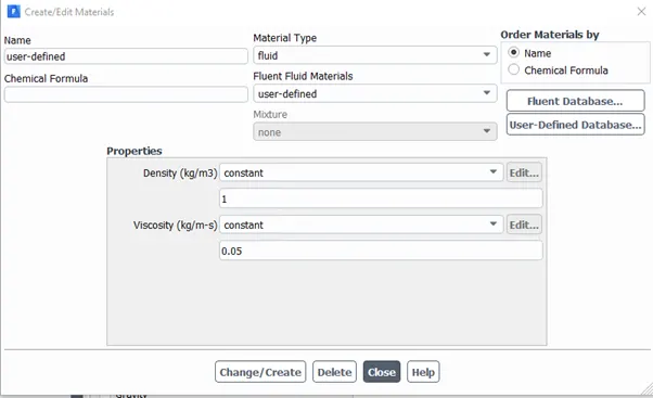
For Materials User defined is provided. The values of density and viscosity are 1kg/m3 and 0.05kg/m-s.
Boundary condition
|
Inlet |
Velocity inlet |
Velocity=0.25m/s |
|
Outlet |
Pressure outlet |
Gauge pressure=0 Pa |
|
Wall |
Wall |
No slip wall |
|
Symmetry |
Symmetry |
symmetry |
The velocity is varied from 0.25,2.5,25,250,2500 based upon the Reynolds number.
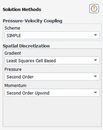
SIMPLE is used under scheme. More quickly convergence can be obtained for relatively simple problems(e.g laminar, where the convergence is limited by the pressure velocity coupling).
Reference Value
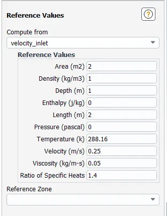
The values of area and length is chosen to be 2. So that the values of drag and lift coefficient will be within the range.
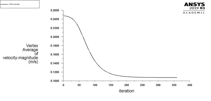
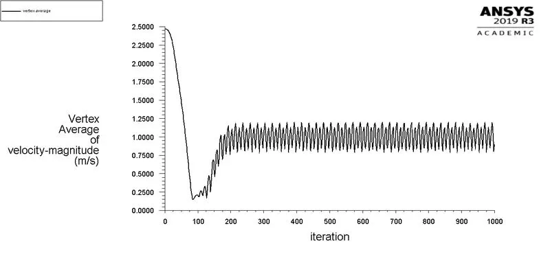
A point is created at a distance of 8m from the wall to measure the vertex average. A plot of Drag, the lift is created under-report definition to measure the coefficient of drag and lift at different iteration/timestep.Hybrid initialization is provided under initialization.
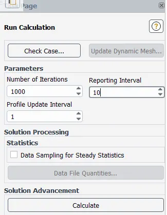
Results and discussion:
Part 1
Simulate the flow with the steady and unsteady case and calculate the Strouhal Number for Re= 100.
By using Theoritical formulae
Strouhal Number= 0.158994
Steady:
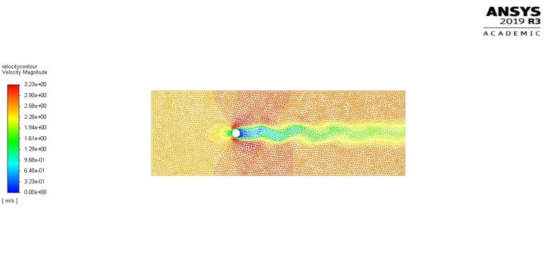
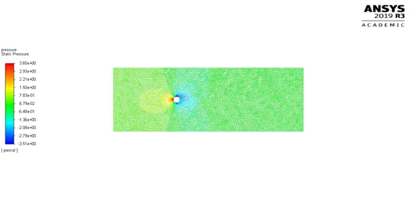
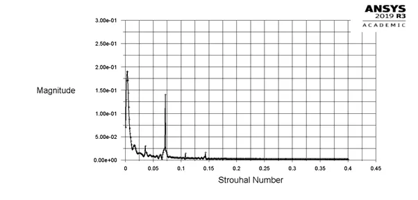
Strouhal Number=0.18971194
Transient:
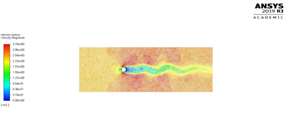
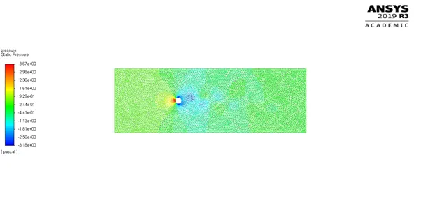
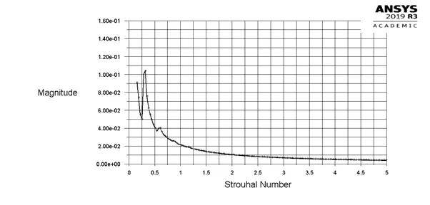
Strouhal Number=0.10396107
There is a 19.32% deviation between theoretical and steady-state analysis. The deviation can be minimized by improving the mesh quality.
Part II
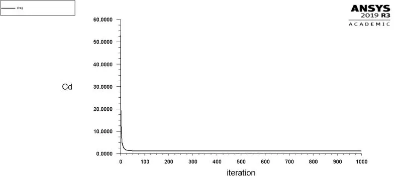
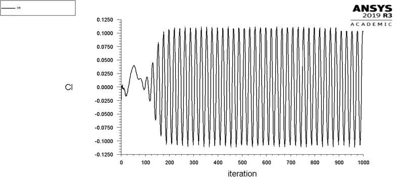
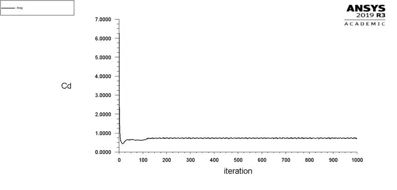
- Calculate the coefficient of drag and lift over a cylinder by setting the Reynolds number to 10,100,1000,10000 & 100000. (Run with steady solver)
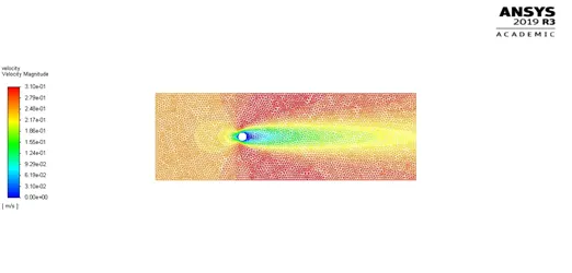
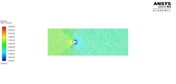
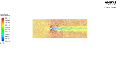
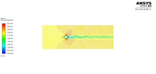
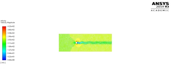
Velocity Contour and Pressure Contour
Re=10
Re=100
Re=1000
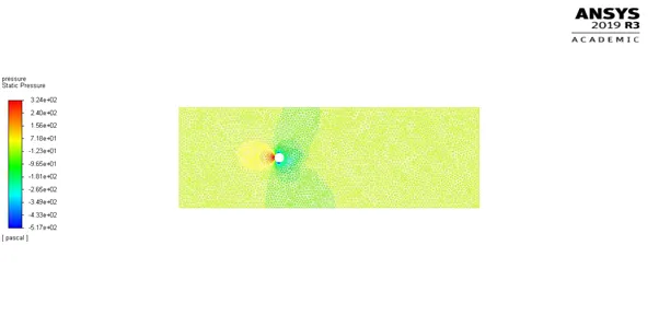
Re=10000
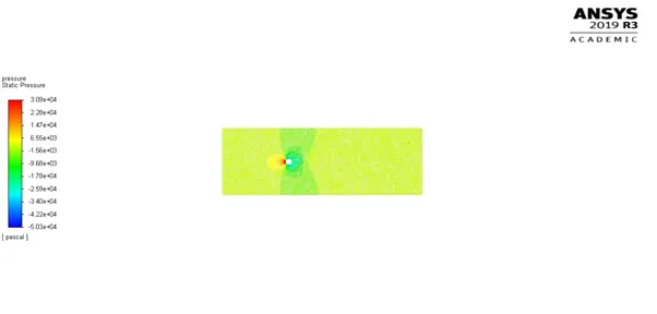
Re=100000
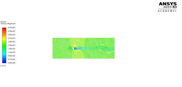
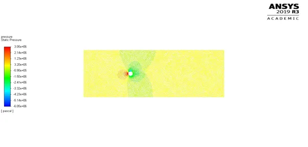
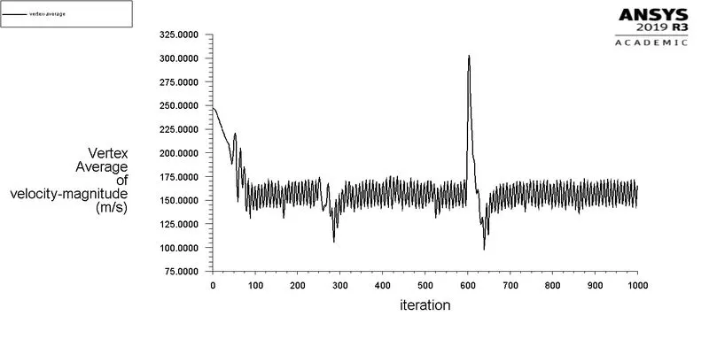
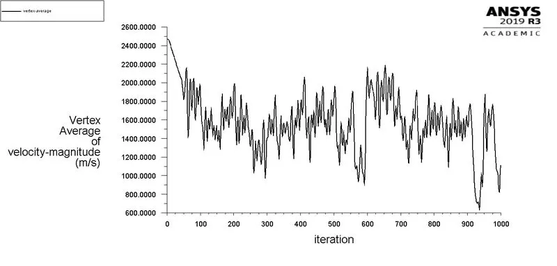
It can be seen from the velocity graph that as the Reynolds number increases the oscillaton dominates the fluid flow
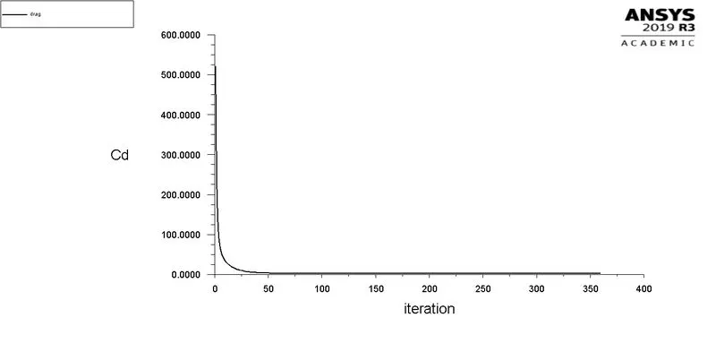
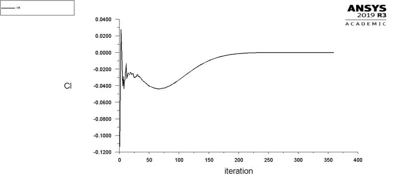
Coefficient of drag and Lift
Re=10
Re=100
Re=1000
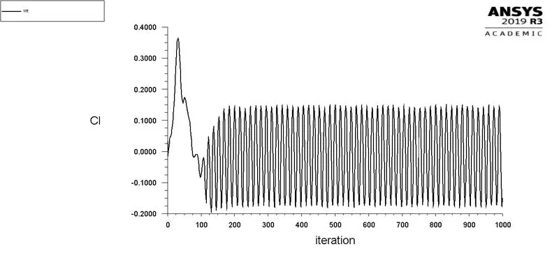
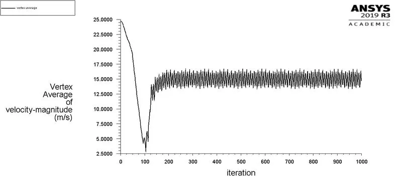
Re=10000
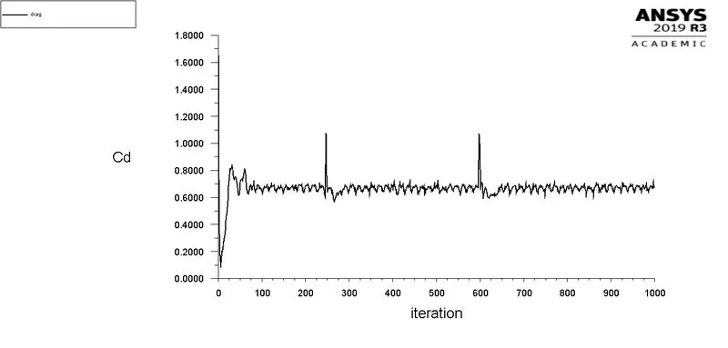
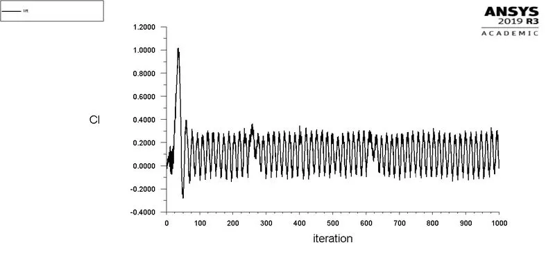
Re=100000
|
Vertex Avg(m/s) |
CI |
CD |
|
|
10 |
0.10770942 |
-6.0235738e-05 |
3.3153958 |
|
100(Steady) |
0.89983916 |
0.1028357 |
1.3212229 |
|
100(Transient) |
0.41167933 |
-0.029792564 |
1.2781799 |
|
1000 |
14.678471 |
-0.14845293 |
0.73358305 |
|
10000 |
165.47087 |
-0.0230036 |
0.67658306 |
|
100000 |
1113.9567 |
0.26024957 |
0.54466477 |
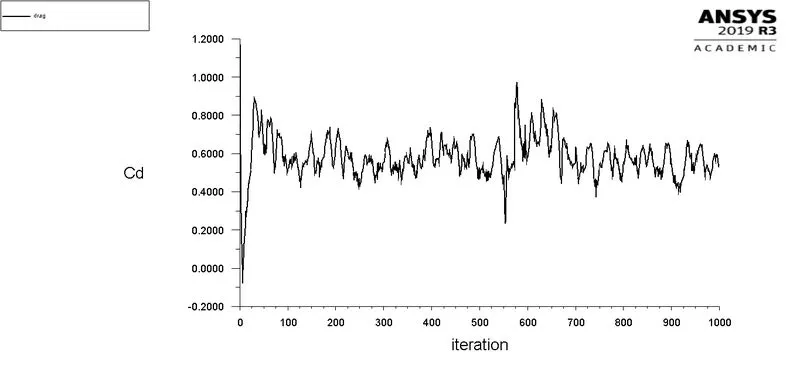
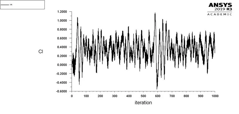
In order to verify the drag coefficient obtained from the ANSYS analysis, solution comparison is made with the research paper[1]. In Article[1] the value for the coefficient of drag at Re=100 is 1.3353 whereas in ANSYS simulation software the value of Cd=1.3212 and the error is within 5%. Hence the obtained solution has the least error and it can be accepted. It can be seen from the graph that as reynolds number increases Coefficient of drag values decreases.
Residual Plot
Re=10
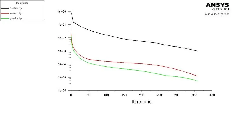
Re=100
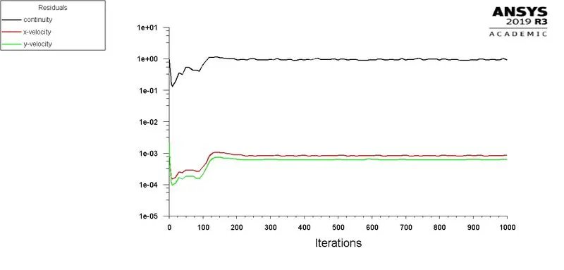
Re=1000
Re=10000
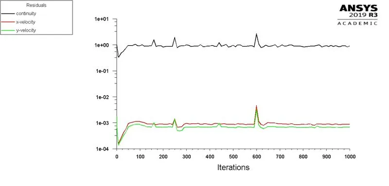
Re=100000
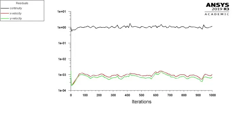
From the iterations plot, it can be inferred that as the Reynolds number increases residue also increases this is due to the presence of oscillation at a higher Reynolds number.
Conclusion
As the Reynolds number increases oscillation dominates the fluid flow and the coefficient of drag is the function of the Reynolds number. As the Reynolds number increases the coefficient of drag decreases which is in accordance with the research paper. The value of vertex average has a direct relationship with the Reynolds number. Frequency of oscillation increases with increase in reynolds number. It is important to design the structural objects such that the frequency of oscillation should not be equal to the resonant frequency.