Week 9 - FVM Literature Review

Finite volume method

Finite volume method is similar to the finite difference method in which the domain is divided into very small elements of geometrically similar shapes. This method is based on the fact that many physical laws are conservation laws. I.e. what goes into one cell on one side leaves the same cell on the other side. This leads to a formulation that consists of flux conservation equation defined in the average sense over the cells. In FVM accuracy is based on the order of the polynomial used.

In FDM it is difficult to satisfy conservation and this method is difficult to apply for complex geometries.

Interpolation schemes

Interpolation schemes are generally used to transform cell centred quantities to the face centred quantities. Linear interpolation is the simplest way of calculating interface values and its gradient. This can be explained by solving the one-dimensional steady-state diffusion problem.

One dimensional steady-state diffusion equation

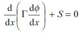
-property it can be temperature, pressure etc

- Diffusion coefficient

S- source term

Grid generation

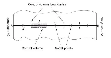
The first major step in FVM is that the domain is divided into discrete control volumes. The control volume at the boundary is determined in such a way that the physical boundaries coincide with the control volume boundaries.

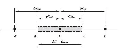
P,W,E-nodal points

e- East face of the CV

w- West face of the CV

Discretisation

The governing equation is integrated over its control volume to yield a discretised equations at its nodal points.

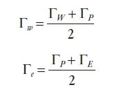
From this equation, it can be concluded that the discretised equation automatically satisfies the conservation equation ie the diffusive flux entering the east face minus the diffusive flux leaving the west face is equal to the source term. In order to derive useful forms of the discretised equation the interface diffusion coefficient and the gradient at the east and west faces of the CV are required. Generally, the valuesand are calculated at the nodal points. In order to find these values at the faces of the CV, Linear interpolation scheme is used. By using the central differencing approach the updated diffusion coefficients are

The gradient term becomes

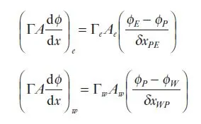
By substituting the updated values of the diffusion coefficient and gradients in the above-discretised equation, the equation becomes

The above equation can be written as

This equation can be converted into an algebraic equation by substituting the constant values and the change in properties are calculated thought the domain by solving the algebraic equations.

Flux limiters

Flux Limiters are used to give physically realisable and meaningful values by limiting the spatial derivative to realistic values. They are used to avoid wiggles that occur during the higher-order discretization schemes, discontinuities in the solution domain and so on.