Week 2 - Flow over a Cylinder.
AIM: Flow over a cylinder and explain the phenomena of von karman vertex street under the steady and unstedy state condition.Calculate the coefficient of Drag and lift for the diffrent value of reynolds number.
PROBLEM STATEMENT:
PART-I
- Simulate the flow with the steady and unsteady case and calculate the Strouhal Number for Re= 100.
PART-II
- Calculate the coefficient of drag and lift over a cylinder by setting the Reynolds number to 10,100,1000,10000 & 100000. (Run with steady solver)
- Discuss the effect of Reynolds number on the coefficient of drag. [ Results should be validated with any standard literature and error should be within 5 %]
INTRODUCTION THEORY:
Von karman vertex street :
In fluid dynamics, a von Karman street is a repeating pattern of swirling vortices caused by a process known as vortex shedding, which is responsible for the unsteady separation of flow of a fluid around blunt bodies.
vortex shedding is an oscillating flow that takes place when a fluid such as air or water flows past a bluff body at certain velocities, depending on the size and shape of the body.in this flow, vortices are created at the back of the body and detach periodically from either side of the body forming von Karman vortex street. the fluid flow past the object creates alternating low-pressure vortices on the downstream of the object. the object will tend to move toward the low-pressure zone.
When the body experiences the pressure drag during the fluid movement, then the body is said to blunt. They are said to have separated flow over a considerable portion of its layer.
Flow separation:
When a fluid is forced to flow over a curved surface at high velocities a fluid follows the front portion of the curved surface with no problem but it has difficulty remaining attached to the surface on the back side. At sufficiently high velocities, the fluid strem detaches itself from the surface of the body this is called as flow separation.
The location of the separation depends upon the sevaral factors such as reynolds number the surface roughness and the level of fluctuations in the free stream,and the level of fluctuations in the free stream, and it is usually diificult to predict actually where the separation will occur unless there are sharp corners or abrupt changes in the shape of solid surface.
> High viscoscity fluids will generate low wake region in comparision to low viscocity fluids.
PROCEDURE:
GEOMETRY:
> open spaceclaim
> use circle tool and teh create a circle atorigin.
> Use construction line and then draw the line with respect to the given dimension.
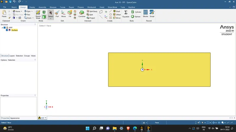
> After that use Reactangle tool and then create a reactangle of size 60*20 m.
> use pull command to convert the 1D geometry in to 2D geometry.
> Use pull command and then select the 1D geometry.
> After selecting the geometry (reactangle), the 1D object will get converted in to 2D.
> select the inner circle and then delete the inner circle.
MESHING:
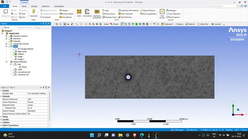
Mesh method: all triangles (second order)
number of division about the edge of the cylinder: 36
Inflation layer :
FLT=5mm
growth rate =1.2
no of layers=6
inflation Layer and the number of divisions are used to capture the circular geometry so that nodes can calculate values.
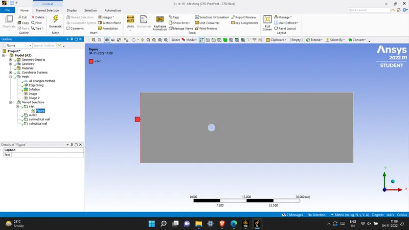
> Inlet
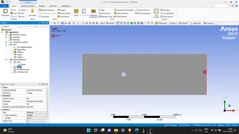
> Outlet
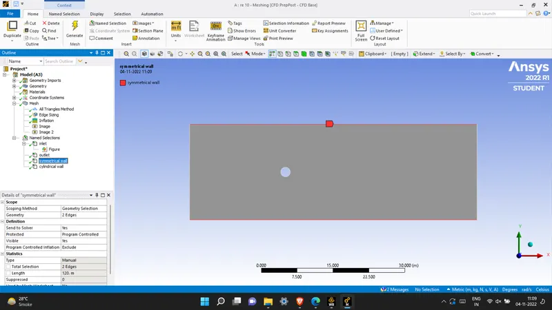
> symmetrical wall
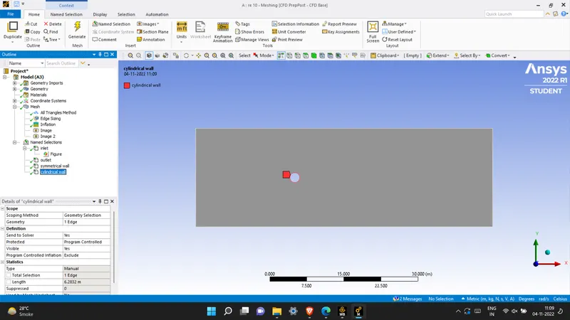
> Cylindrical wall
FLUENT SETUP:
CASE 1 : Steady state solver with reynolds number of 100.
| SOLVER | STEADY STATE,PRESSURE BASED |
| METHOD | SIMPLE |
| VELOCITY FORMULTION | ABSOLUTE |
| ENERGY EQUATIONS | OFF |
| VISCOUS MODEL | LAMINAR |
| INLET | VELOCITY INLET |
| OUTLET | PRESSURE OUTLET |
| MATERIAL | USER DEFINED WITH DENSITY AS 1 AND DYNAMIC VISCOSITY OF 0.05 |
BOUNDARY CONDITIONS
inlet v=2.5 ms-1
no slip condition for wall
and 0 gauge pressure for the outlet
Monitor point is at a distance 8 units from the origin. (origin is the centre of the cylinder)
BY SIMPLE solution method and Hybrid initialization we solve the problem.
A) STEADY CASE
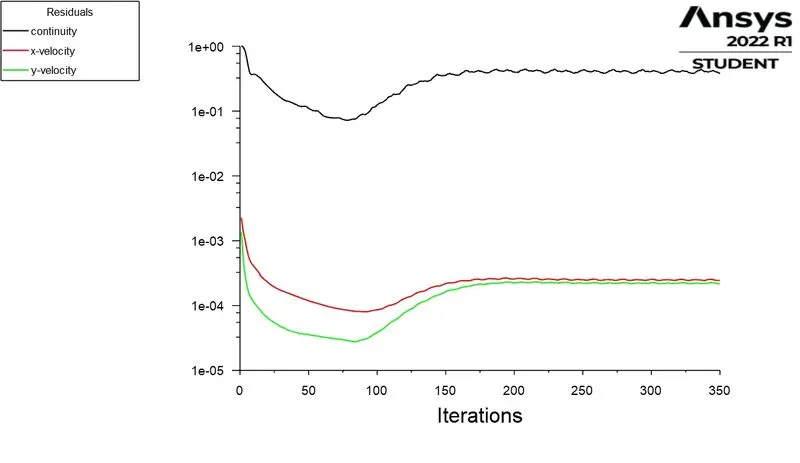
Scaled residuals:
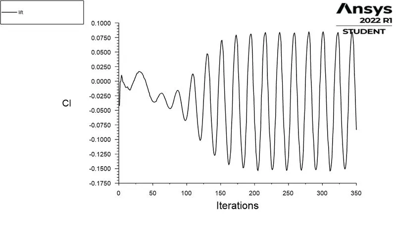
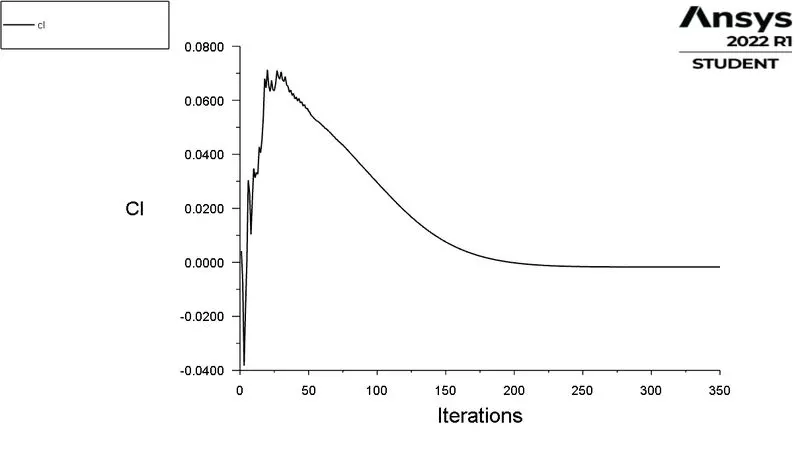
Lift :
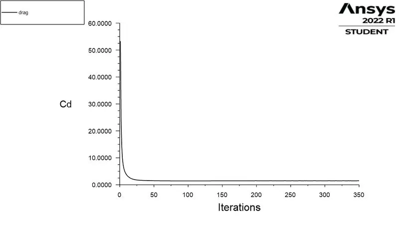
Drag:
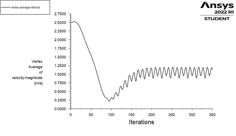
> vertex average velocity:
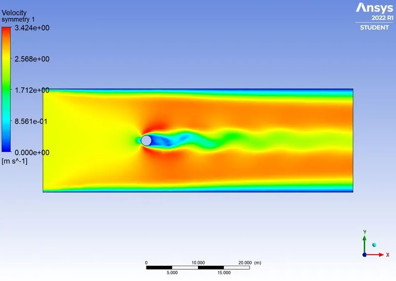
Velocity contour:
Pressure contour:
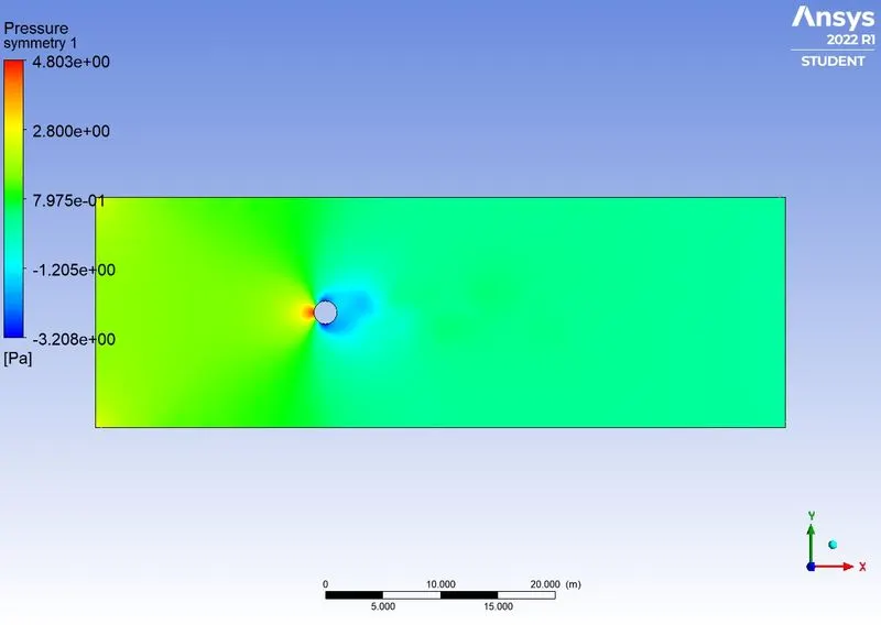
we cant find Strouhal number for steady flow condition as it represents the ratio of inertial forces due to unsteadiness of the flow or local acceleration to the inertial forces due to change in velocity in flow field.
> VIDEO ANIMATION OF THE VELOCITY CONTOUR FOR THE STEADY FLOW WITH REYNOLDS NUMBER 100.
https://www.youtube.com/watch?v=kXC1Wef5IqY
B) CASE 2 : Unsteady state solver with reynolds number of 100.
|
SOLVER |
UNSTEADY STATE,PRESSURE BASED |
|
Time step size |
0.1 second |
| Number of iterations | 1000 |
| METHOD | SIMPLE |
| VELOCITY FORMULATION | ABSOLUTE |
| ENERGY EQUATIONS | OFF |
| VISCOUS MODEL | LAMINAR |
| INLET | VELOCITY INLET |
| OUTLET | PRESSURE OUTLET |
|
MATERIAL |
USER DEFINED WITH DENSITY AS 1 AND DYNAMIC VISCOSITY OF 0.05 |
BOUNDARY CONDITIONS
inlet v=2.5ms-1
no slip condition for wall
and 0 gauge pressure for the outlet
Monitor point is at a distance 8 units from the origin. (origin is the centre of the cylinder)
BY SIMPLE solution method and Hybrid initialization we solve the problem.
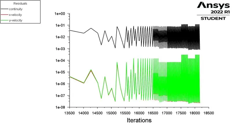
> SCALED RESIDUAL:
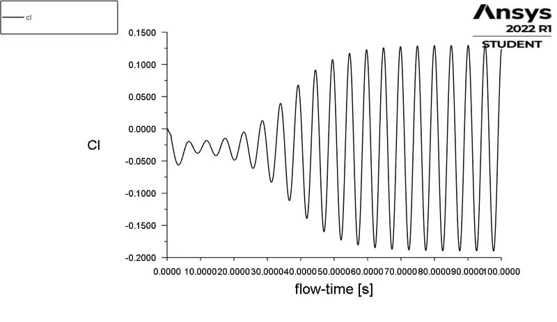
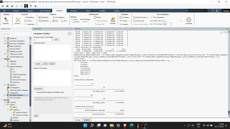
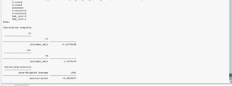
Results – Lift and Drag Coefficients.
• Both the lift and drag coefficients fluctuate periodically with time. Because the vortex shedding alternates on either
side of the cylinder, the lift force (represented by the lift coefficient in the plot below) varies between positive and
negative peaks in a sinusoidal manner. The positive peak corresponds to the vortex shed on the upper side, and the
negative peak – to the vortex shed on the lower side. The period equals to the time between vortex shedding on
the same side.
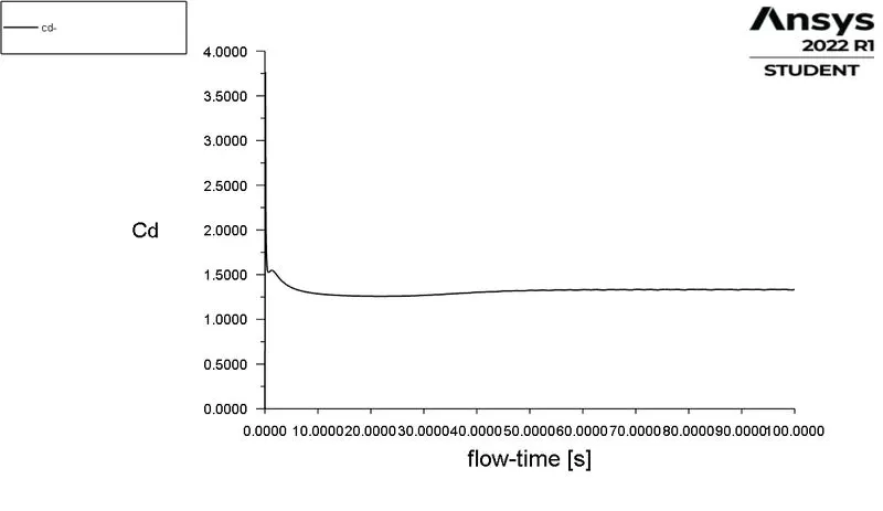
• The drag force (represented by its coefficient) oscillated at half the period of the lift force, as both vortices shed
from the top and bottom induce the drag force in the same direction. Unlike lift, the drag force is always positive
> LIFT:
DRAG:
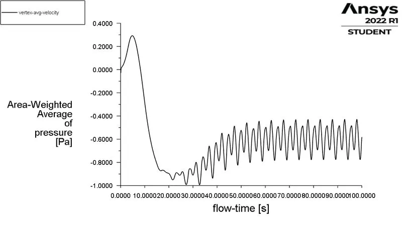
> vertex average velocity for Re 100 unsteady.
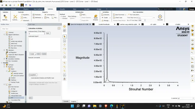
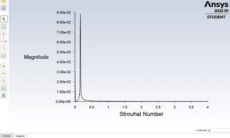
> STROUHAL NUMBER:
vertex shedding frequency F can be calculated using the graph
strouhal number :- St=F⋅LV">St=(F⋅L)/V
where F is vertex shedding frequency
L is characteristic length or diameter
v is the velocity of the moving fluid.
How to calculate strouhal number??
Solution > Results > plot > FFT > y-axis function as magnitude > x-axis function as strouhal number > load input file > select lift profile > plot fft > x-axis label as strouhal number > x axis variation as iterations > y axis label as Magnitude > y-axis variable as lift > write fft to file .
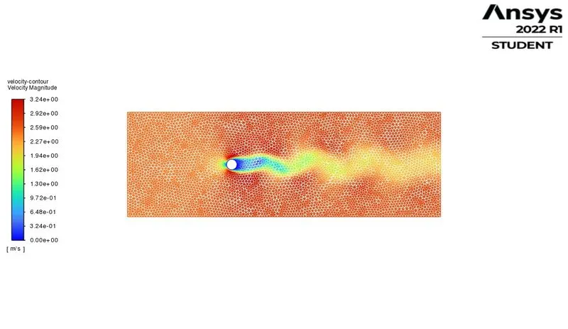
> Velocity contour:
The vortex shedding takes place when the water flows past the cylinder at a certain range of Reynolds Numbers.
• In this example, the global Reynolds Number (𝑅𝑒𝐷 = 𝜌𝑉𝐷Τ𝜇) is approximately 100, corresponding to periodic
unsteady vortex shedding flow regime.
• Vortices are formed behind the cylinder and detach periodically from either side. Then the alternating vortices
travel along with the main flow towards the downstream region, forming a von Kármán vortex street
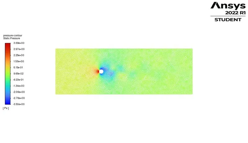
> Pressure contour:
• Vortices, characterized by low pressures at their cores, propagate downstream with the flow.
• The periodic alternation of high and low pressures at either side of the cylinder results in periodic forces acting
on the cylinder in both the horizontal (drag force) and vertical (lift force) directions.
> VIDEO ANIMATION OF THE VELOCITY CONTOUR FOR THE UNSTEADY FLOW WITH REYNOLDS NUMBER 100.
https://youtu.be/W4z9aCtS4E8
OBSERVATIONS AND CONVERGENCE
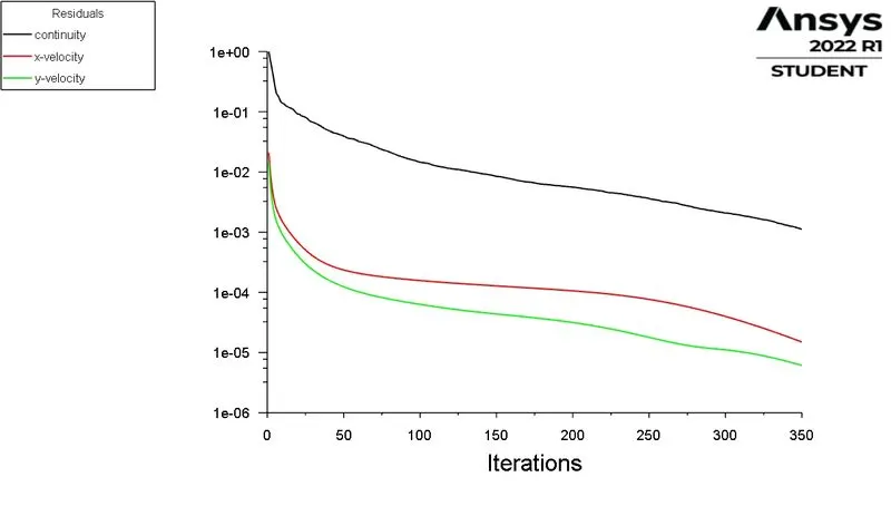
- From the residual plot, we can see that the flow has converged around 350 iterations in the steady case and 18000 iterations in an unsteady state.
- The vorticity can be considered as a local measure of the spinning motion of a fluid, which is often used to visualize the vortices or eddies .
- In the residual plot the continuity and value of X and Y become stable which means flow has converged.
- Steady flow results give the final results, while in the unsteady flow it gives results based on flow time.
- Unsteady analysis can give accurate solutions of vertices and shedding frequency and we can get intermediary results.
- When your simulation has no change on all the convergence criteria, after certain iterations or timesteps, then we can consider that the solution has reached a steady-state, i.e.., converged.
- In convergence, there is no change after some iterations or they follow the same pattern
CASE 4: STEADY STATE SIMULATION RE 10
| SOLVER | STEADY STATE,PRESSURE BASED |
| METHOD | SIMPLE |
| VELOCITY FORMULTION | ABSOLUTE |
| ENERGY EQUATIONS | OFF |
| VISCOUS MODEL | LAMINAR |
| INLET | VELOCITY INLET |
| OUTLET | PRESSURE OUTLET |
| MATERIAL | USER DEFINED WITH DENSITY AS 1 AND DYNAMIC VISCOSITY OF 0.05 |
BOUNDARY CONDITIONS
inlet v= 0.25 ms-1
no slip coition for wall
and 0 gauge pressure for the outlet
Monitor point is at a distance 8 units from the origin. (origin is the centre of the cylinder)
BY SIMPLE solution method and Hybrid initialization we solve the problem.
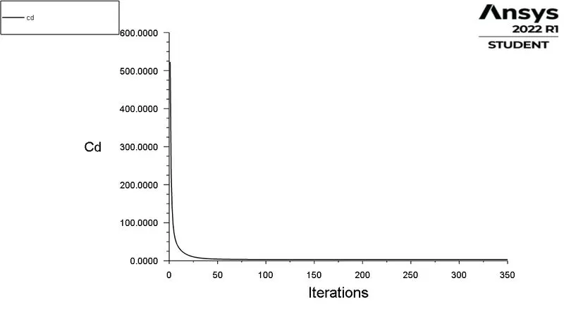
SCALED RESIDUALS:
> LIFT:
> DRAG:
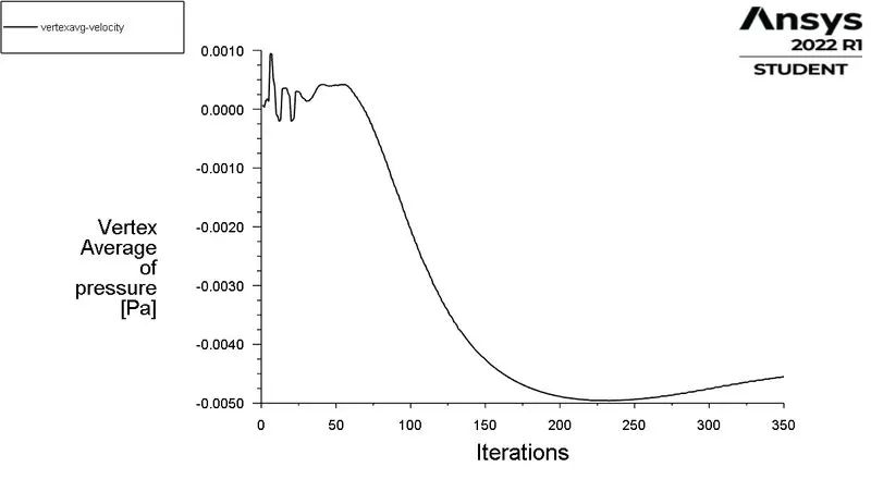
>VERTEX AVERAGE VELOCITY:

POST PROCESSING:
VELOCITY CONTOUR:
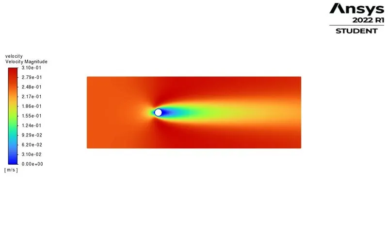
There is no formation of von karman vertex street at the reynold number 10.
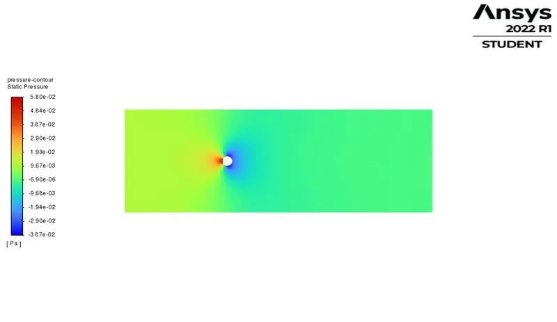
> PRESSURE CONTOUR:
CASE 3 : Steady state solver with reynold number of 1000
| SOLVER | STEADY STATE,PRESSURE BASED |
| METHOD | SIMPLE |
| VELOCITY FORMULTION | ABSOLUTE |
| ENERGY EQUATIONS | OFF |
| VISCOUS MODEL | LAMINAR |
| INLET | VELOCITY INLET |
| OUTLET | PRESSURE OUTLET |
| MATERIAL | USER DEFINED WITH DENSITY AS 1 AND DYNAMIC VISCOSITY OF 0.05 |
BOUNDARY CONDITIONS
inlet v= 25 ms-1
no slip coition for wall
and 0 gauge pressure for the outlet
Monitor point is at a distance 8 units from the origin. (origin is the centre of the cylinder)
BY SIMPLE solution method and Hybrid initialization we solve the problem.
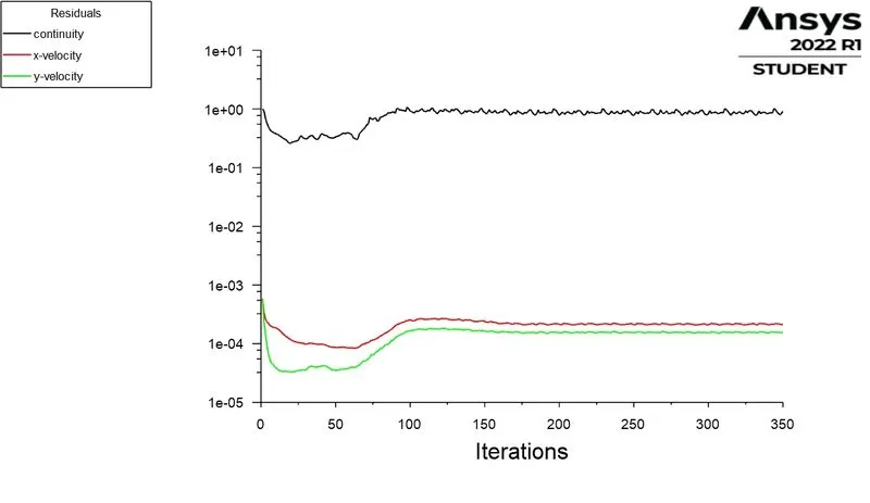
SCALED RESIDUALS:
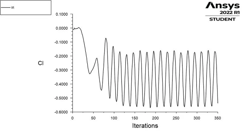
> LIFT:
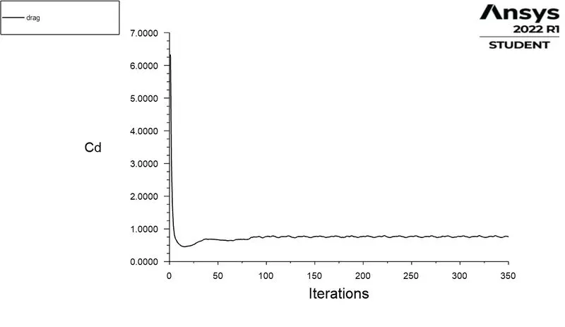
> DRAG:
POST-PROCESSING:
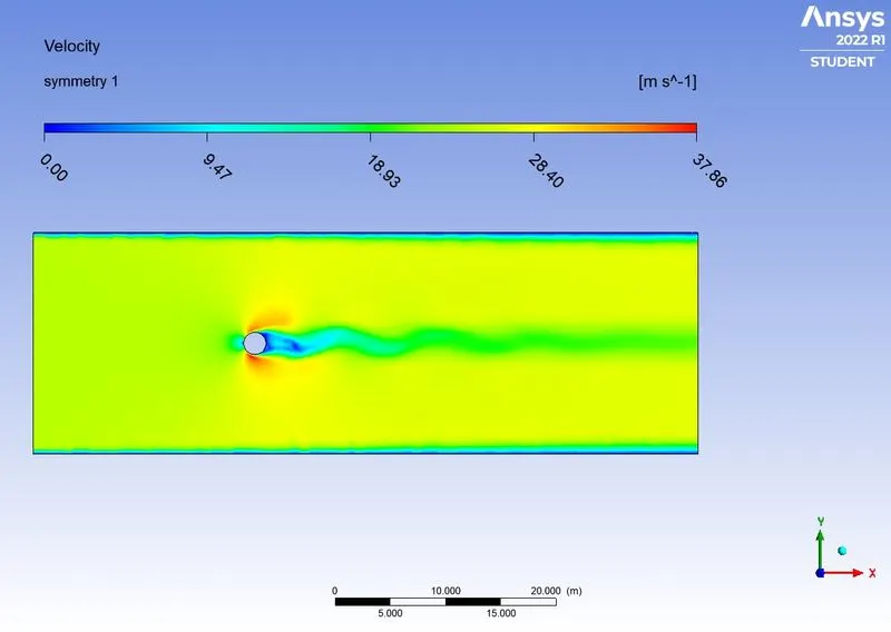
> VELOCITY CONTOUR:
> PRESSURE CONTOUR:
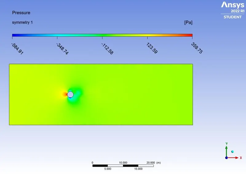
> VIDEO ANIMATION OF THE VELOCITY CONTOUR FOR THE STEADY FLOW WITH REYNOLDS NUMBER 1000.
https://youtu.be/YuuaD523R-4
CASE 4 : Steady state solver with reynold number of 10000
| SOLVER | STEADY STATE,PRESSURE BASED |
| METHOD | SIMPLE |
| VELOCITY FORMULTION | ABSOLUTE |
| ENERGY EQUATIONS | OFF |
| VISCOUS MODEL | LAMINAR |
| INLET | VELOCITY INLET |
| OUTLET | PRESSURE OUTLET |
| MATERIAL | USER DEFINED WITH DENSITY AS 1 AND DYNAMIC VISCOSITY OF 0.05 |
BOUNDARY CONDITIONS
inlet v= 250 ms-1
no slip coition for wall
and 0 gauge pressure for the outlet
Monitor point is at a distance 8 units from the origin. (origin is the centre of the cylinder)
BY SIMPLE solution method and Hybrid initialization we solve the problem.
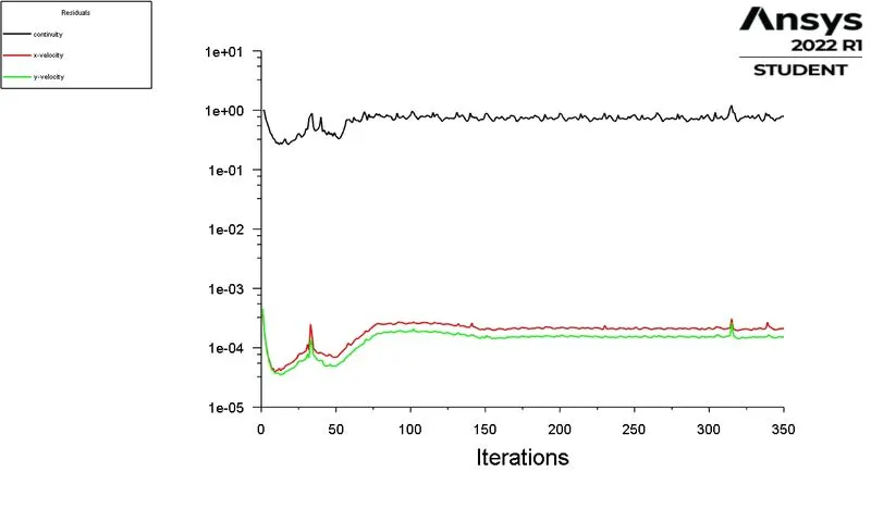
> Scaled residuals:
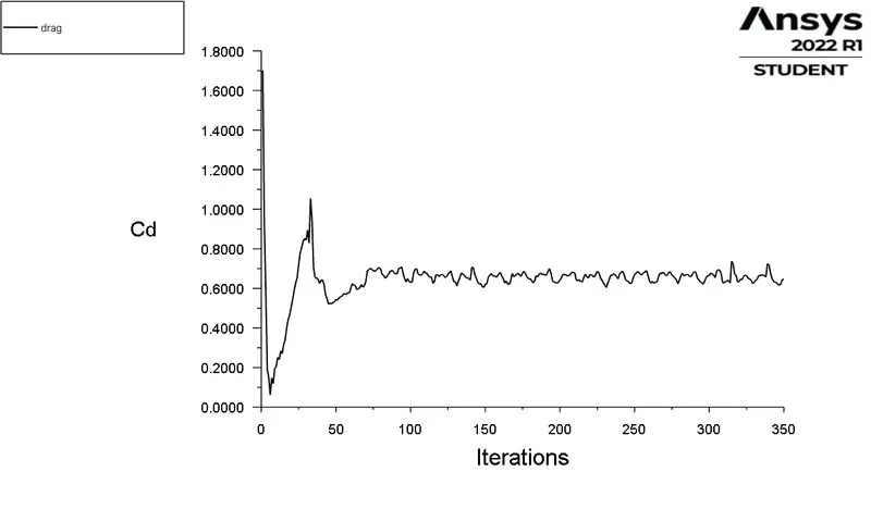
> Drag:
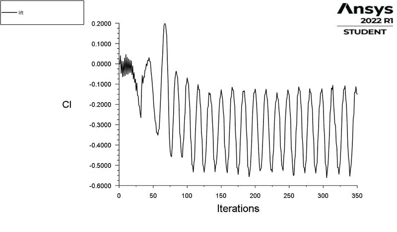
> Lift:
> Vertex average velocity for Re 10000.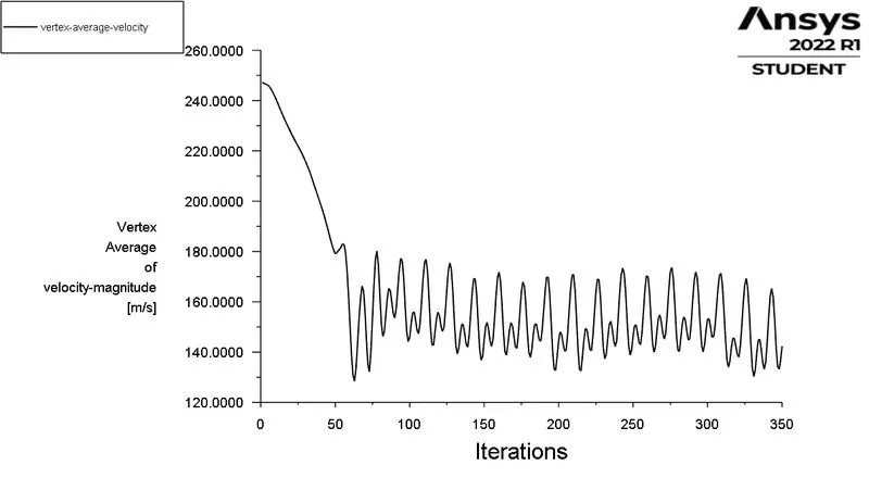
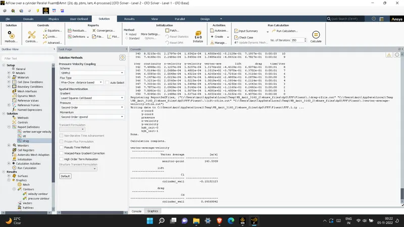

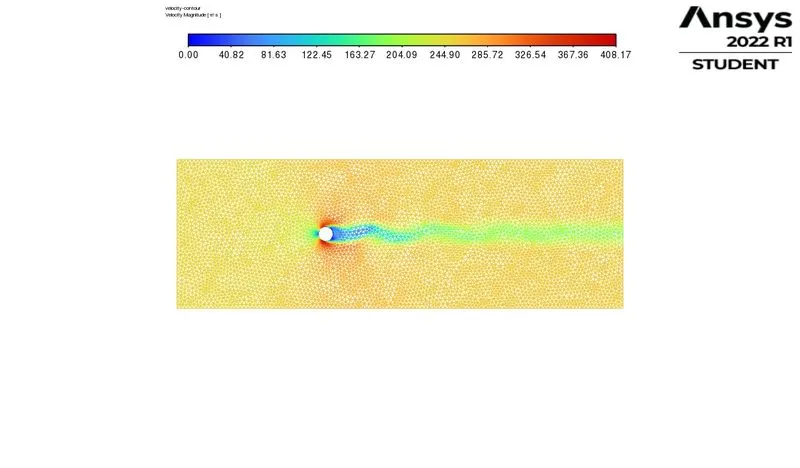
POST PROCESSING:
VELOCITY CONTOUR:
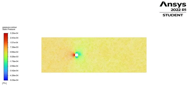
> PRESSURE CONTOUR:
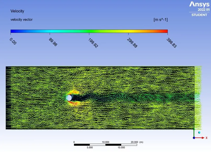
> VELOCITY VECTOR:
CASE 4:
| SOLVER | STEADY STATE,PRESSURE BASED |
| METHOD | SIMPLE |
| VELOCITY FORMULTION | ABSOLUTE |
| ENERGY EQUATIONS | OFF |
| VISCOUS MODEL | LAMINAR |
| INLET | VELOCITY INLET |
| OUTLET | PRESSURE OUTLET |
| MATERIAL | USER DEFINED WITH DENSITY AS 1 AND DYNAMIC VISCOSITY OF 0.05 |
BOUNDARY CONDITIONS
inlet v= 2500 ms-1
no slip coition for wall
and 0 gauge pressure for the outlet
Monitor point is at a distance 8 units from the origin. (origin is the centre of the cylinder)
BY SIMPLE solution method and Hybrid initialization we solve the problem.
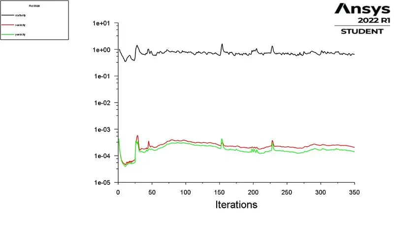
> Scaled Residuals:
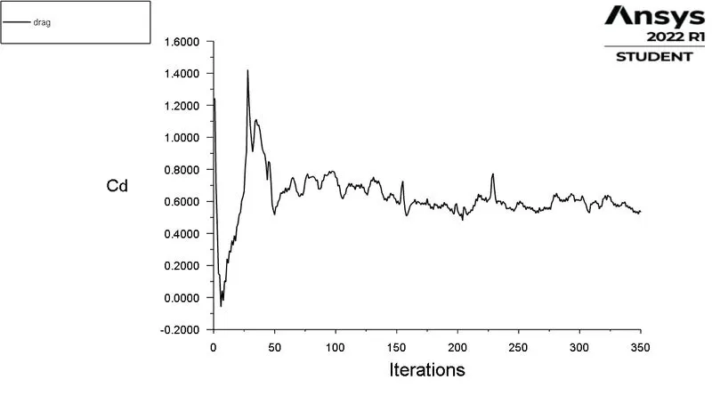
> DRAG:
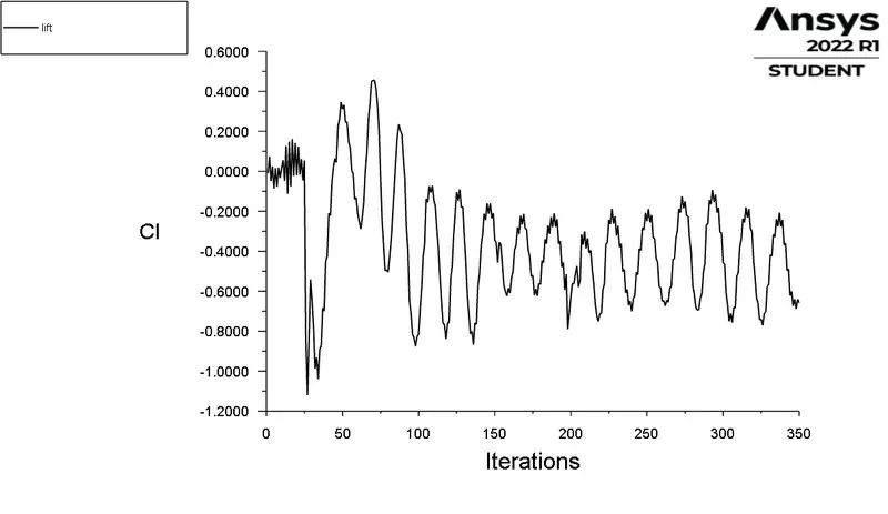
> LIFT:
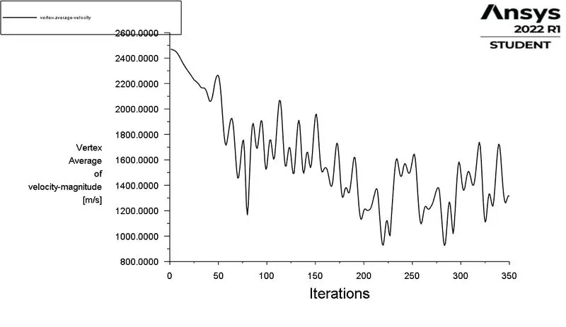
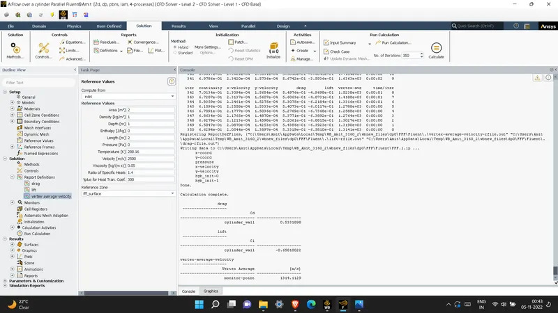
>VORTEX AVERAGE VELOCITY:

POST PROCESSING :
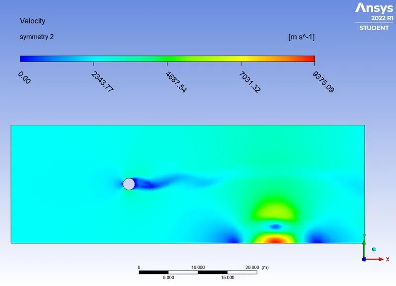
velocity contour:
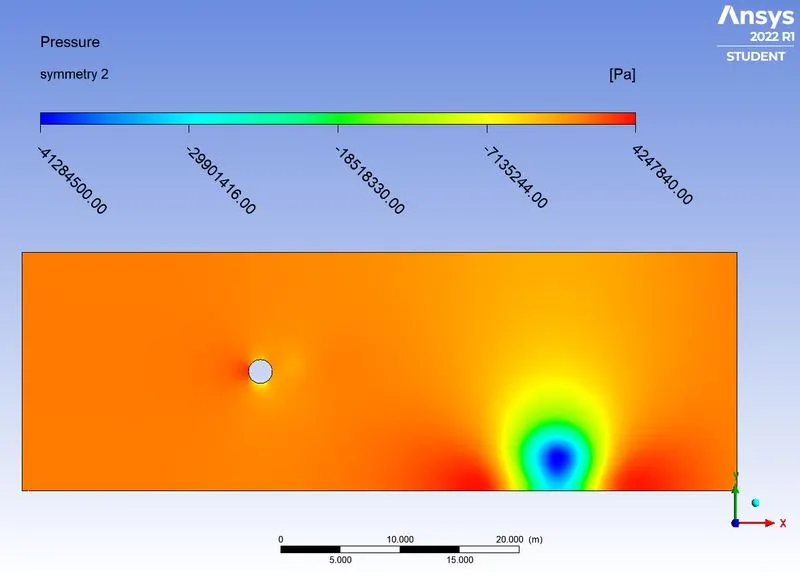
> Pressure contour:
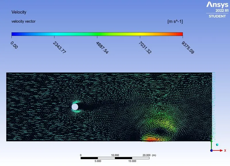
> velocity vector:
CONCLUSION
- with an increase in Reynolds\'s number the drag coefficient increases.
- flow pattern becomes unsymmetrical wrt to the axis perpendicular to the flow
- drag force is inversely proportional to Reynolds numbers for (Re<300 where the flow is laminar after that it gets converted to turbulent ) if we change dynamic viscosity.
references:
> Ansys fluent
unsteady flow over a cylinder - simulation example
> wikipedia
> science direct research paper