Week 2 - Flow over a Cylinder.
Flow over a Cylinder
Aim
- Simulate the flow with the steady and unsteady case and calculate the Strouhal Number for Re= 100.
- Calculate the coefficient of drag and lift over a cylinder by setting the Reynolds number to 10,100,1000,10000 & 100000. (Run with steady solver)
- Discuss the effect of Reynolds number on the coefficient of drag. [ Results should be validated with any standard literature and error should be within 5 %]
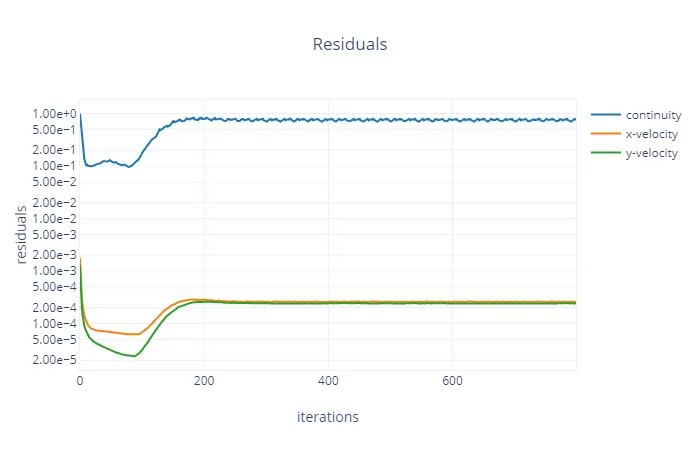
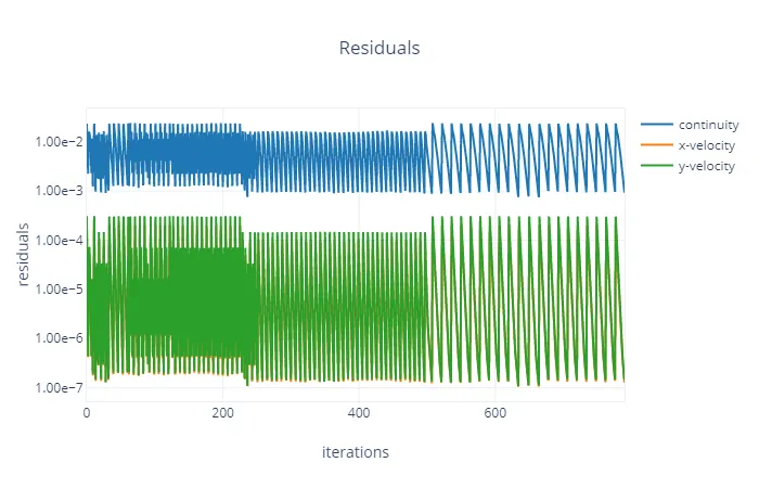
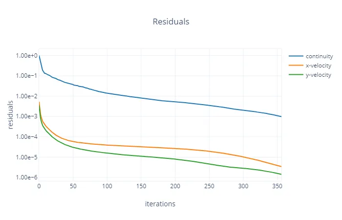
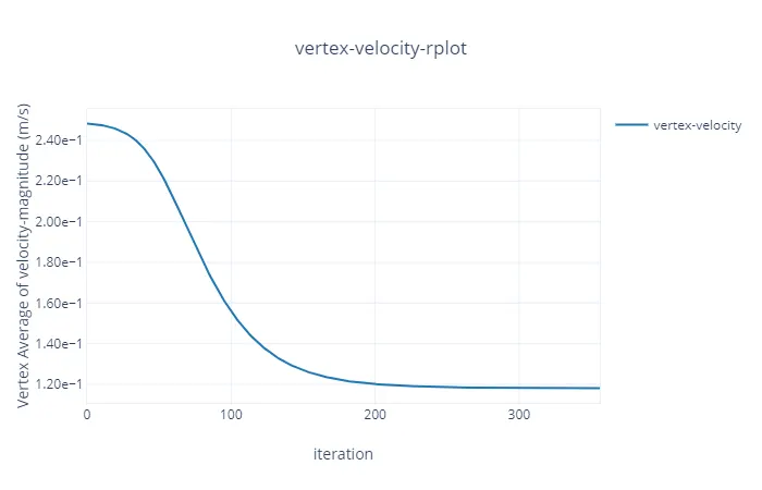
- In both approaches, show that the flow has converged. That is, what quantities or plots need to be looked at to determine that the flow has converged?
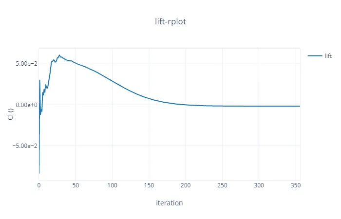
- Plots of the coefficient of drag and lift.
- Plots to show vortex shedding behind the cylinder.
- Mention the referred material (Reference Paper or Fluid Mechanics Textbook) at the end of the challenge submission page.
Introduction
Flow over cylinder:
In spite of extensive experimental and numerical studies almost over a century, flow around a circular cylinder still remains a challenging problem in fluid mechanics, where intensive investigations are continued even today to understand the complex unsteady dynamics of the cylinder wake flow. Cross-flow normal to the axis of a stationary circular cylinder and the associated problems of heat and mass transport are encountered in a
wide variety of engineering applications. Both experimental measurements and numerical computations have confirmed the onset of instability of the wake flow behind a cylinder beyond a critical Reynolds number, leading finally to a kind of periodic flow identified by definite frequencies, well-known in the literature as the Von Karman vortex street. In case of laminar flow past cylinders with regular polygonal cross-section, the flow
usually separates at one or more sharp corners of the cross-section geometry itself, forming a system of vortices in the wake on either side of the mid symmetry plane. On the other hand, for a circular cylinder, where the point of flow separation is decided by the nature of the upstream boundary layer, the physics of the flow is much more complex than what its relatively simple shape might suggest.
Theory
VISCOUS FLOW
When the molecules move from one location to another, they transport their mass, momentum, and energy in the fluid and gives rise to mass diffusion, viscosity (friction), and thermal conduction. A flow where the viscous forces are present is known as the viscous flow. Friction forces are acting between the fluid layers. Reynolds number is finite for viscous flow. Practically, all the flows are viscous flow only, no matter how small may be the magnitude of the force but it is present.
In viscous flow, the velocity at the surface of the body will be zero. Due to the presence of the viscosity, there will be a difference in the pressure distribution and also shear stress will vary along the body. Therefore, the net unbalanced forces will not be zero and the body will produce aerodynamic forces such as lift and drag. The pressure around the surface of the body will not be distributed symmetrically since velocity will change along the streamlines. Mass diffusion and thermal conduction will occur among the particles.
Reynolds Number (Re):
Reynolds number for a flow is a measure of the ratio of inertial to viscous forces in the flow of a fluid around a body.
Re = rho*V*d/Dynamic Viscosity
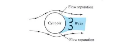
The range of Re values will vary with the size and shape of the body from which the eddies are being shed, as well as with the kinematic viscosity of the fluid. Over a large Red range (47<Red<105 for circular cylinders; reference length is d: diameter of the circular cylinder) eddies are shed continuously from each side of the circle boundary, forming rows of vortices in its wake. The alternation leads to the core of a vortex in one row being opposite the point midway between two vortex cores in the other row, giving rise to the distinctive pattern shown in the picture. Ultimately, the energy of the vortices is consumed by viscosity as they move further downstream, and the regular pattern disappears.
Strouhal number (St):
Strouhal number is a dimensionless number describing oscillating flow mechanisms.
The Strouhal number is often given as
St = f*d/u
Where,
f is the frequency of vortex shading,
L is the characteristic length and
U is the flow velocity.
Solving & Modelling approach
Simulate the flow over a cylinder and explain the phenomenon of Karman vortex street.
PART-I
- Simulate the flow with the steady and unsteady case and calculate the Strouhal Number for Re= 100.
PART-II
- Calculate the coefficient of drag and lift over a cylinder by setting the Reynolds number to 10,100,1000,10000 & 100000. (Run with steady solver)
- Discuss the effect of Reynolds number on the coefficient of drag. [ Results should be validated with any standard literature and error should be within 5 %]
Pre-processing and solver setting
Geometry
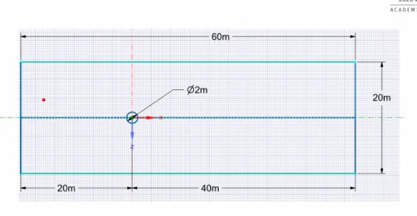
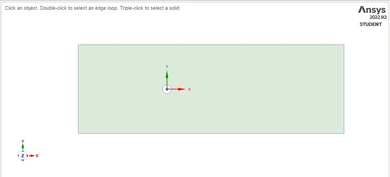
change the view to x-y plane ansd select the sketch module for creating the geometry create a circle in the center of the plane with that draw line with line tool and rectangule to create the computational domain PULL TOOL is used create new surface and delete the inner volume of the cylinder
MESH
create a gradual mesh over the domain and generate it and gadualy reduce the traget length upto 500mm and triangular method mesh created and increase the number of division over the cylinder wall to capture tyhe curve and create and infulation layer over the cylinder wall to caputre te boudary layer effect for that first layer thickness and 5.mm and and the number of layer is 6 the growth factor is 1.2
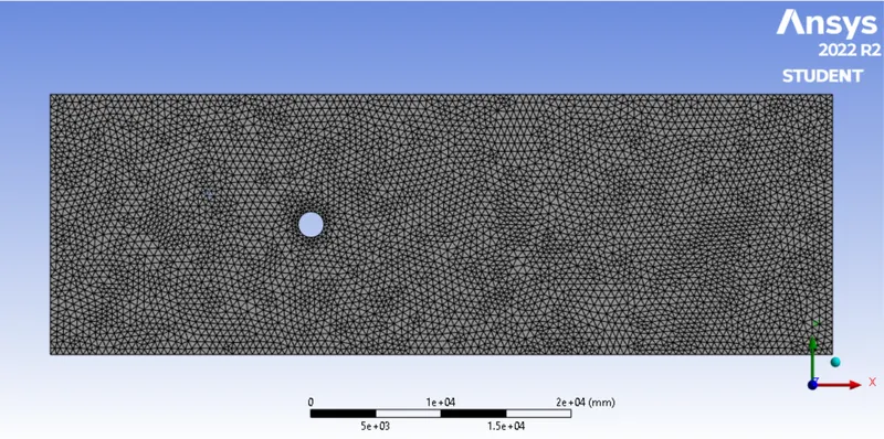
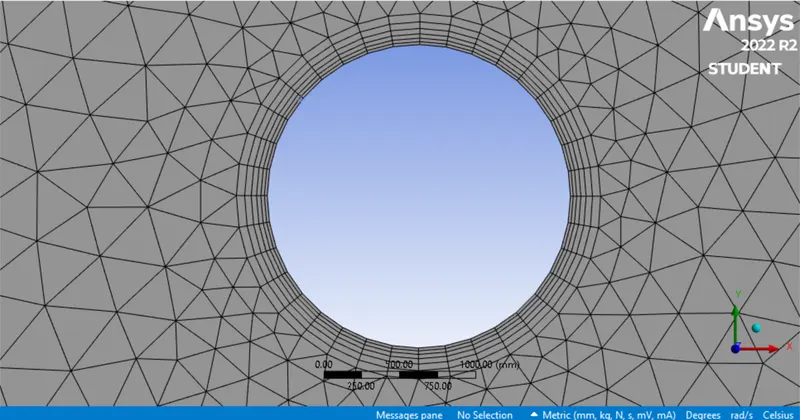
And create the name for the boundary for given boundary condition
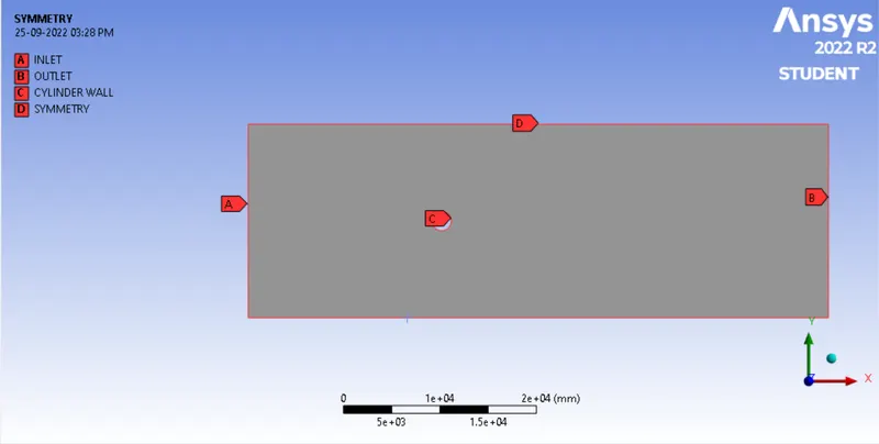
SETUP
Right click ---> edit to fluent setup
General ----> Solver Type ----> preasure Based solver ------> Time ---> steady State
VISCOUS MODELS ---> LAMINAR ---->Standard---.> standard Wall Function
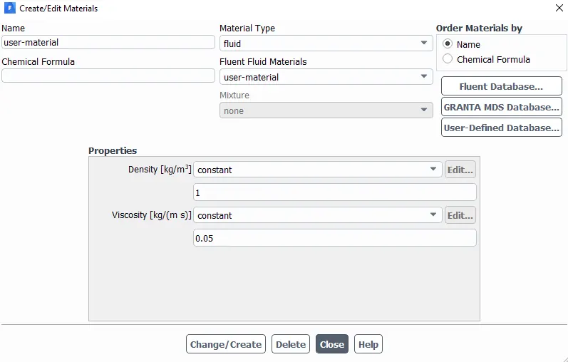
MATERIALS --- > FLUID ----> Air ------>
BOUNDRY CONDTION
INLET -------> VELOCITY INLET (for all cases )
OUTLET ------ -> PRESSURE OUTLET
WALL --------> CYLINDER WALL
OUTLET -----> PRSSURE OUTLET
REFERANCE VALUE --- > Compute for inlet
SOLUTION
METHODE --- > SIMPLE SCHEME
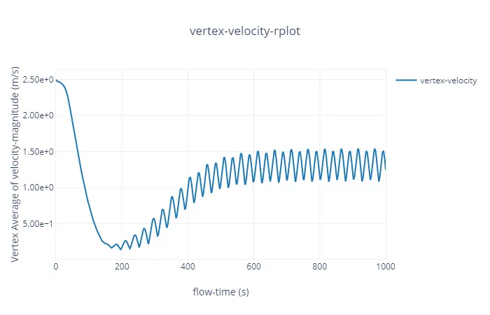
create a moniter point from the center to right side 8m to capture the vortex street
and create residual for the lift and Drag coefficent
PART -1
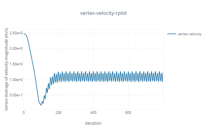
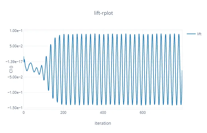
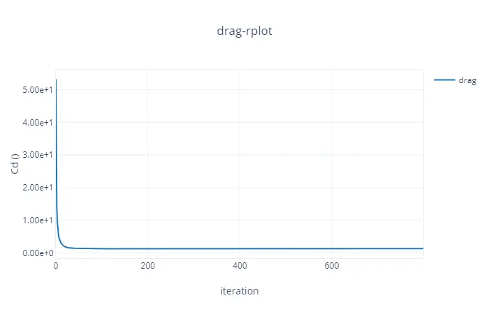
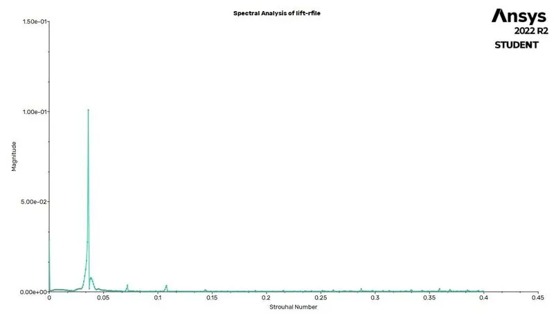
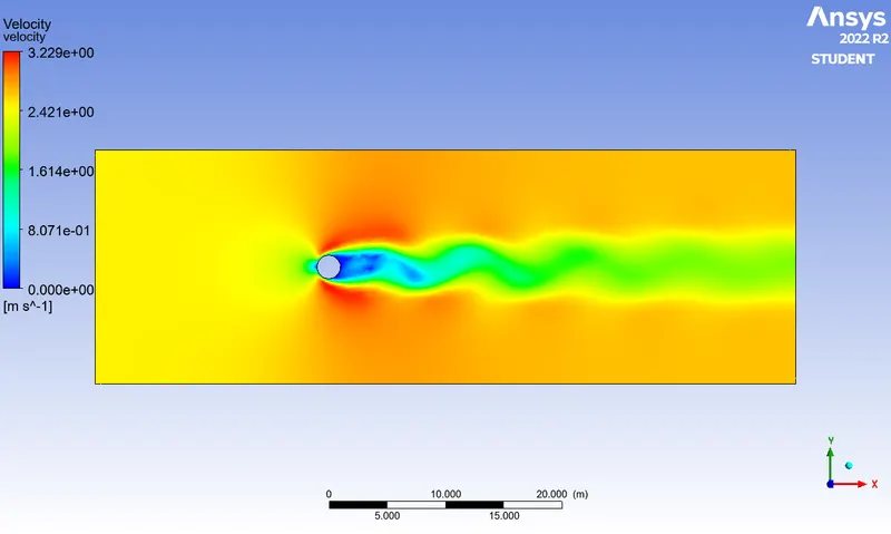
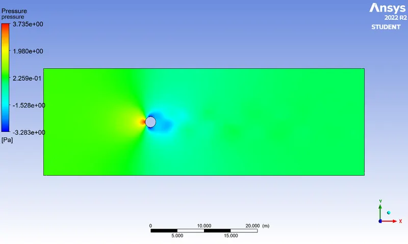
Simulate the flow with the steady case and calculate the Strouhal number for Re=100 and velocity 2.5m/s.
RESIDUALS PLOT
VORTEX VELOCITY
COEFFICIENT OF LIFT
COEFFICIENT OF DRAG
STROUHAL NUMBER PLOT
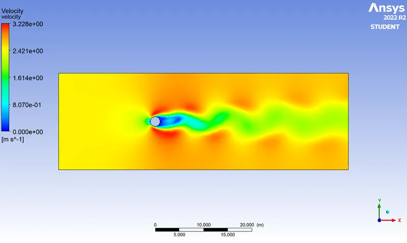
VELOCITY CONTOUR
PRESSURE CONTOUR
ii) Simulate the flow with the unsteady case and calculate the Strouhal number for Re=100 and velocity 2.5m/s.
RESIDUALS PLOT
VORTEX VELOCITY
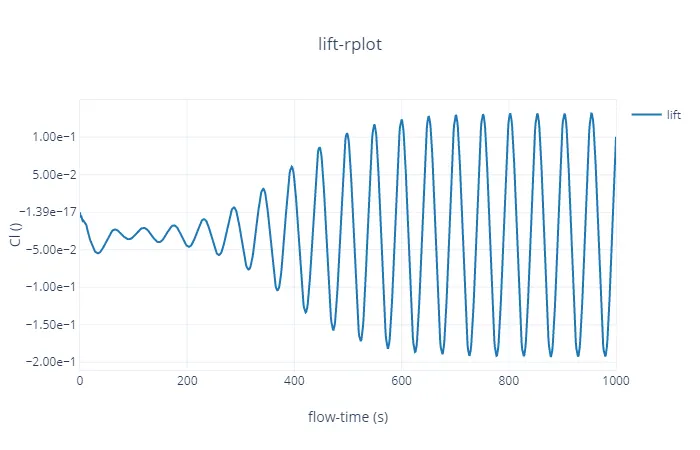
COEFFICIENT OF LIFT
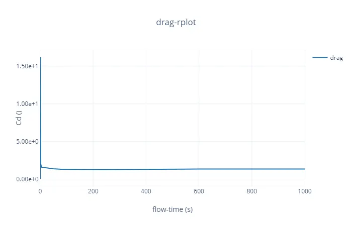
COEFFICIENT OF DRAG
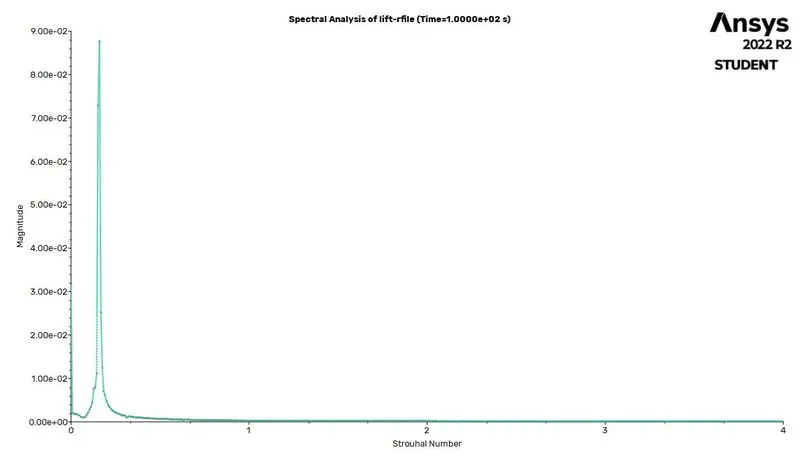
STROUHAL NUMBER PLOT
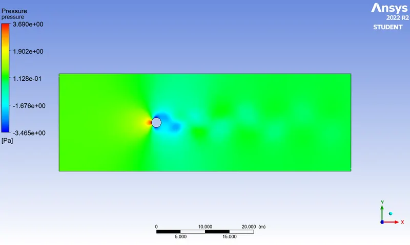
PRESSURE CONTOUR
VELOCITY CONTOUR
Part-2
i) Simulate the flow with the steady-state solver for Re=10.
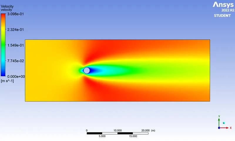
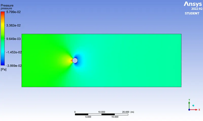
For Re=10 velocity v=0.25m/s
RESIDUALS PLOT
VORTEX VELOCITY
LIFT COEFFICIENT
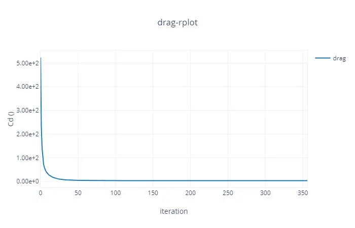
DRAG COEFFICIENT
VELOCITY CONTOUR
PRESSURE CONTOUR
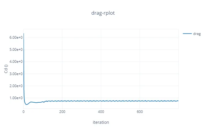
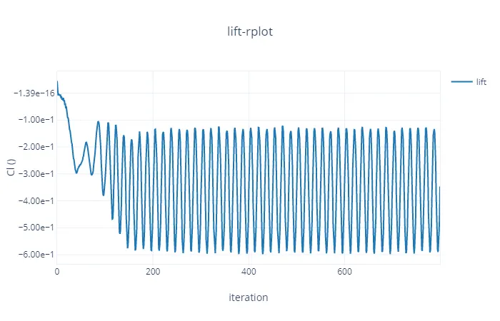
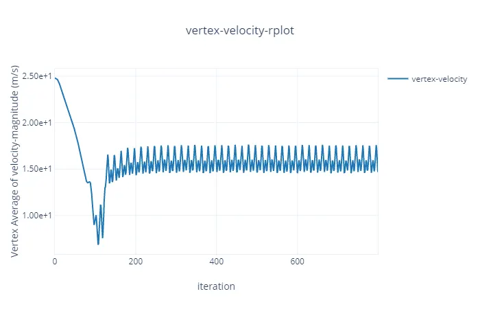
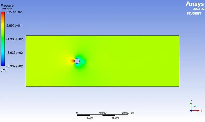
Simulate the flow with the steady-state solver for Re=1000.
For Re=1000 velocity v=25m/s
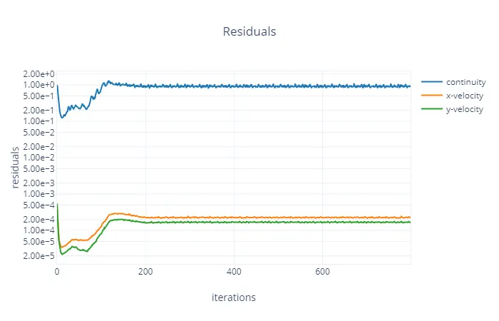
RESIDUAL PLOT
DRAG COEFFICIENT
LIFT COEFFICIENT
VELOCITY VORTEX
PRESSURE CONTOUR
VELOCITY CONTOUR
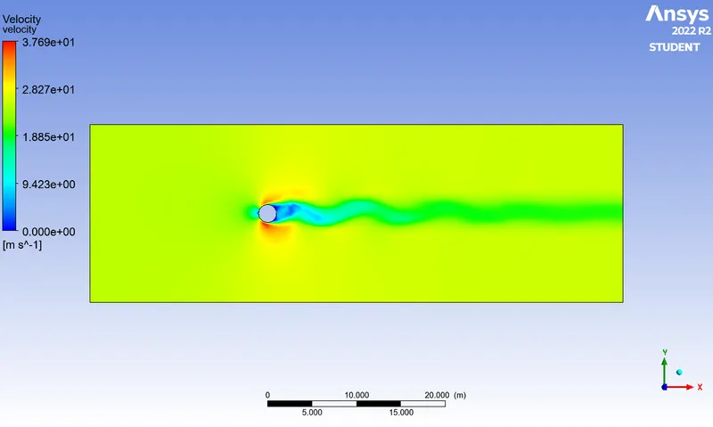
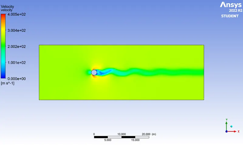
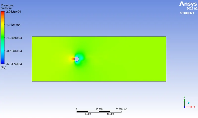
Simulate the flow with the steady-state solver for Re=10000.
For Re=10000 velocity v=250m/s
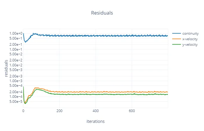
RESIDUALS PLOT
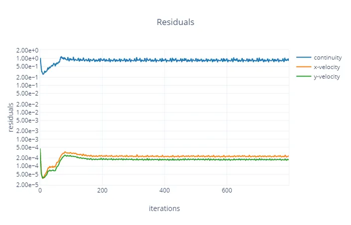
VORTEX VELOCITY
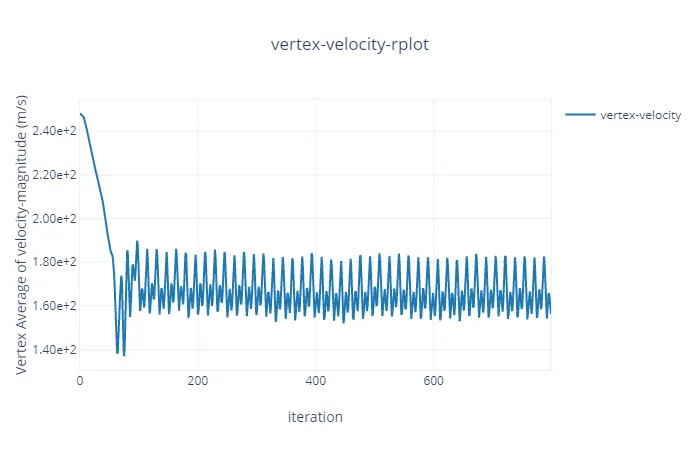
COEFFICIENT LIFT
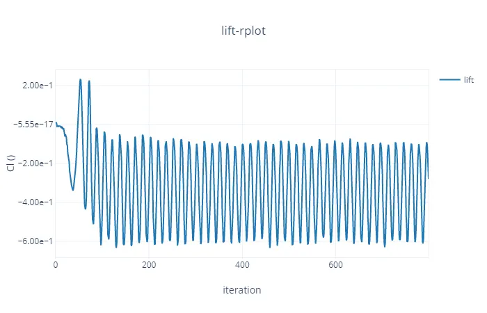
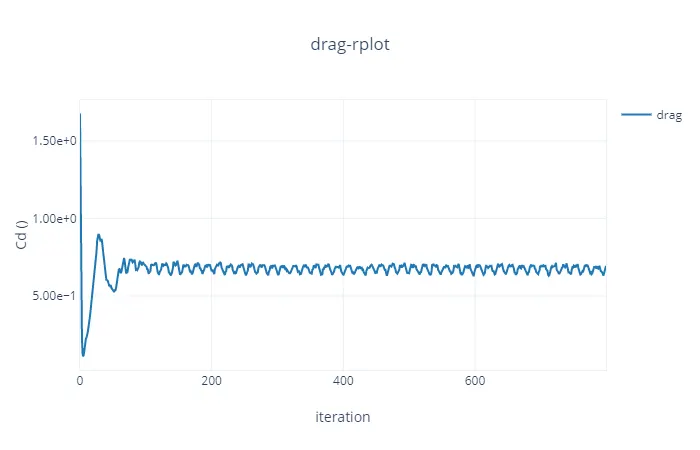
COEFFICIENT OF DRAG
VELOCITY CONTOUR
PRSSURE CONTOUR
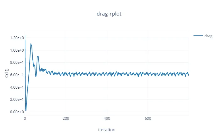
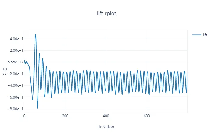
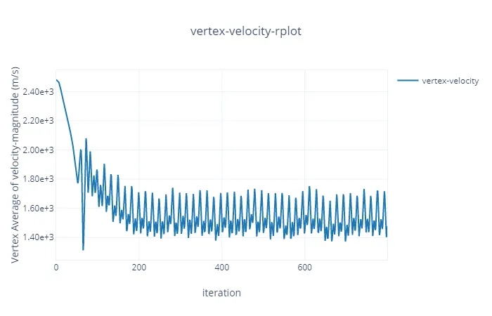
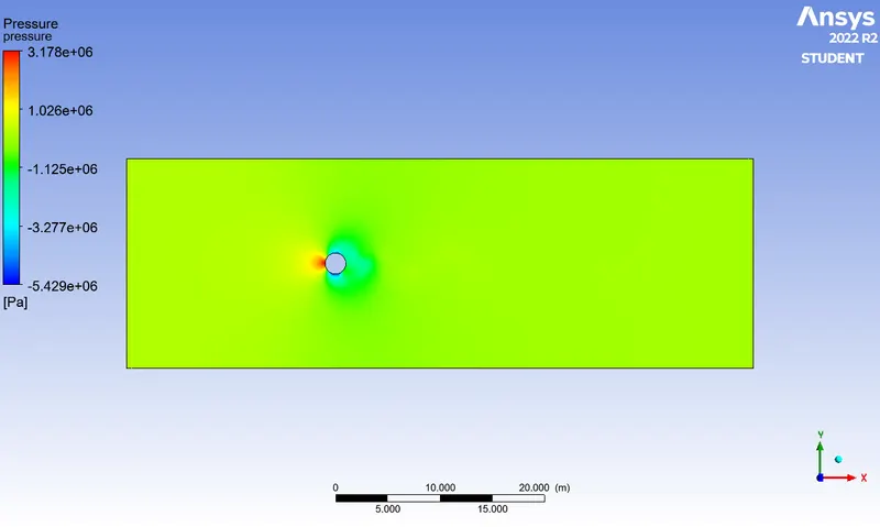
Simulate the flow with the steady-state solver for Re=100000.
For Re=100000 velocity v=2500m/s
RESIDUALS
DRAG COEFFICIENT
 \
\
LIFT COEFFICIENT
VELOCITY VORTEX
PRESSURE CONTOUR
VELOCITY CONTOUR
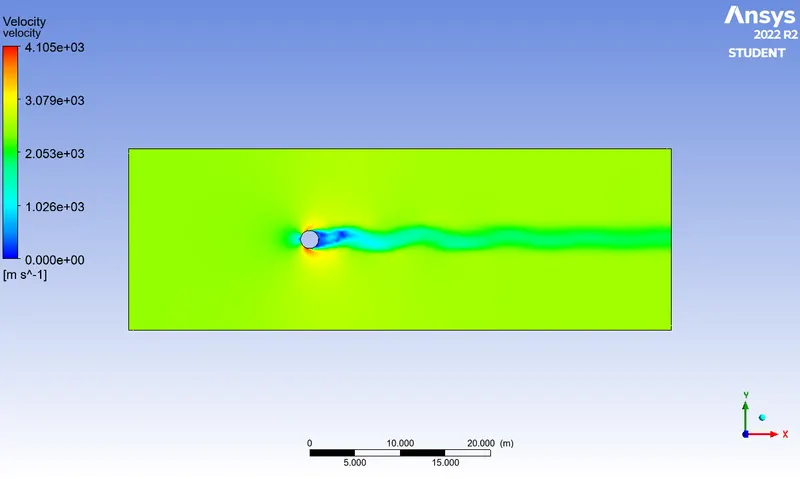
Result:
Drag and lift coefficient for different Re
| Re | Cd | CL |
| 10 | 3.33 | -0.0016 |
| 100 | 1.365 | -0.02 |
| 1000 | 0.736 | -0.34 |
| 10000 | 0.69 | -0.27 |
| 100000 | 0.5867 | -0.1825 |
.Error wrt the theoretical values from the reference material,
| Reynolds number | CL | CD | St | theoritical Cd | error | |
| 100 STEADY | 0.02 | 1.33 | 0.4 | 1.4 | 4.6% | |
| 100 UNSTEADY | 0.1 | 1.33 | 3.99 | 1.4 | 3.6% |
Conclusions:
In the first case, the flow over a cylinder is simulated for both Steady and unsteady cases with Re=100, and with the results generated the phenomena of Von Karman Vortex Street are also observed. Necessary plots are plotted in order to observe that the flow is converged and the vortex shedding is happening. Contours are generated in order to observe the flow over a cylinder. By plotting Power Spectral Density vs Frequency, the Strouhal number is calculated.
In the second case, six different simulations i.e (Re = 10,100,1000,10000,100000,1000000) are simulated to observe the behavior of the drag and lift coefficients by changing the Reynolds number. In order to observe the behavior of the drag coefficients for the simulations, the velocity of the flow is varied to change the Reynolds number and the rest of the parameters are kept constant. As we know if the Reynold number is less than 2000, then flow in a pipe is Laminar. Hence we use the Viscous model = Laminar. For Re=10, it is observed that there is no formation of vortex shedding and in the rest of the cases, it is clearly observed. As per the basic conditions and parameters, the results are validated from the literature. As we refine the mesh we need to run more iterations. From the above table, it can be concluded that the error percentage is less than 5%.
Reference Research Paper:- https://www.sciencedirect.com/science/article/pii/S0307904X08000243