Week 2 - Flow over a Cylinder.
Aim: To simulate the flow over a cylinder and explain the phenomenon of Karman vortex street.
PART-I
- Simulate the flow with the steady and unsteady case and calculate the Strouhal Number for Re= 100.
PART-II
- Calculate the coefficient of drag and lift over a cylinder by setting the Reynolds number to 10,100,1000,10000 & 100000 in steady state.
- Discuss the effect of Reynolds number on the coefficient of drag.
Theory:
Von karman vortex street:
Concept of boundary layer was introduced by Prandtl. When a bluff body is placed in free stream of a fluid flow, when the fluid flows around the cylinder the flow area tend to decrease `(dp)/dx`<0 ie the flow accelerates to a region of low pressure to high pressure. As the flow proceedes it reaches a point where the pressure is minimum subsequently as the flow proceedes gradient of the velocity is zero and thus this point is called separetion point, now as the flow proceedes past a point the flow area tend to increase casusing a decrease in the velocity owing to an increase in the pressure causing `(dp)/dx`>0 an adverse pressure gradient and the velocity decreases leading to formation of eddies.
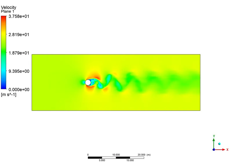
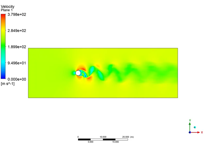
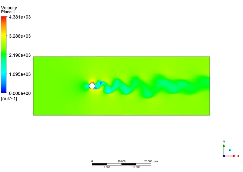
When the flow Reynolds number exceedes 40 the wake behind the cylinder becomes unstable leading to slow oscillations the amplitude of which increases downstream. The oscillating waves rolles up into two staggered rows of vortices having opposite direction. As Re>80 the vortix form close to cylinder and the attathced eddies starts to osscillate and the eddy on one side start to shed during that time the other eddy fprms on the other side and goes on. During this period the cylinder experience an osscillating lift.
Pre-Processing
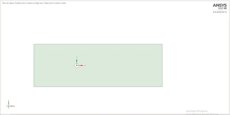
Geometry:
Meshed Geometry:
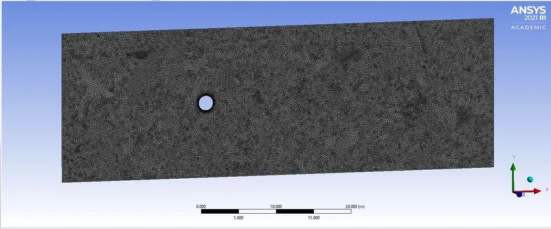
- The geometry was meshed with triangular method with totoal number of elements as 64354
- Edge sizing was given to cylinder with 720 divisions also inflation of 10 layers was added.
Results:
- The simulation was run on pressure based solver under steady condition for Re 10,100,1000,10000,100000
- Also transient state wqas solved for Re = 100
- Material properties was assigned with density of 1kg/m3 and viscocity of 0.05 kg/m.s.
- The Re was increased by varying the velocity keeping the viscocity and density constant.
Part-I
Transient State v/s Steady State
Reynold's number: 100
Flow velocity: 2.5`m/s`
viscocity: 0.05`(kg)/(m*s)`
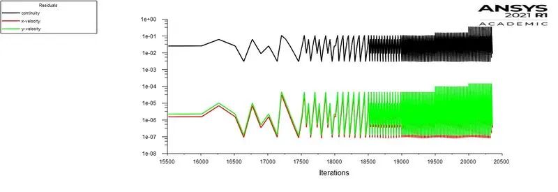
Residual Plot(Transient State):
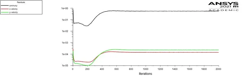
Residual Plot(Steady State):
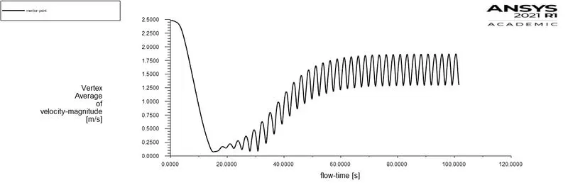
Monitor point velocity(Transient State):
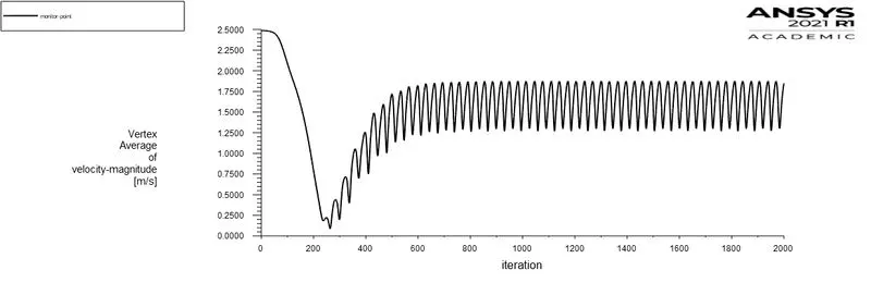
Monitor point velocity(Steady State):
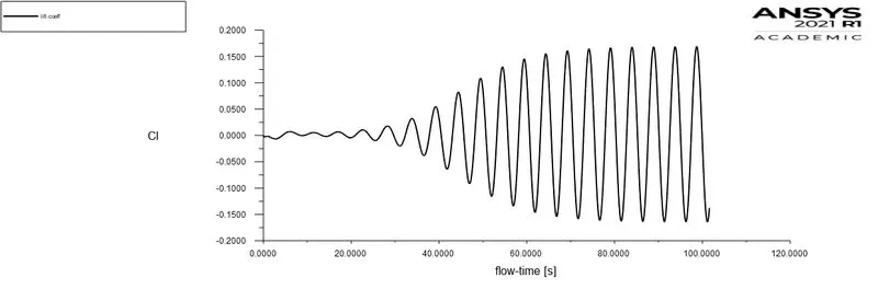
Plot of coefficient of lift(Transient State):
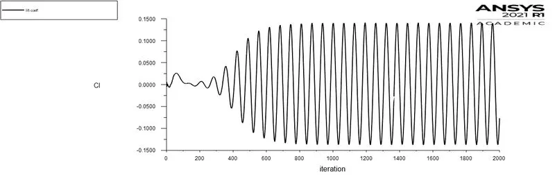
Plot of coefficient of lift(Steady State):
Plot of coefficient of drag(Transient State):
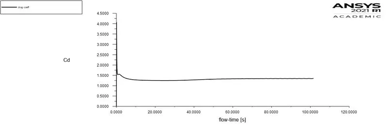
Plot of coefficient of drag(Steady State):
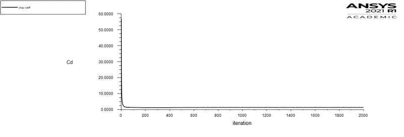
Velocity contour (Transient State):
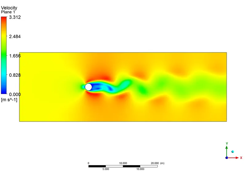
Velocity contour (Steady State):
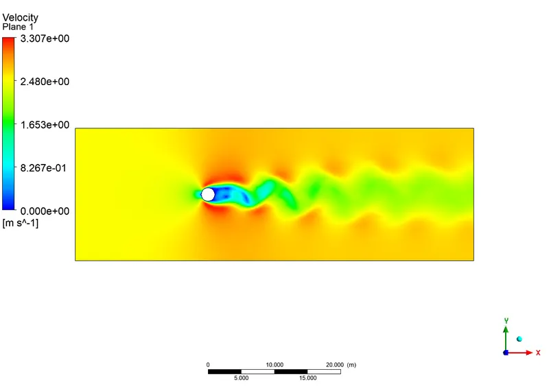
Steady state v/s Transient state
A steady state simulation mainly ignores many of the cross terms and higher order tersms dealing with time. They mainly set these values as zero as they dont affect steady state. Whereas in transient state the simulation include all these terms. hence steady state simluation converges faster when compared to transient.
Strouhal number calculation:
`St = (fL)/U`
`f` = frequency of oscillation.
`f` = `1/(T)`
T = time period
`L` = Projected length of cylinder.
`U` = Free stream velocity.
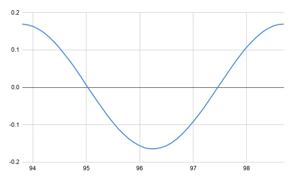
T = `T_2-T_1` = 98.7-93.8
`f` = `(4.9)/1` = 0.0204Hz
U = 2.5m/s
L = 2m
`St` = `(0.204*2)/2.5` = 0.163
Part-II
1. case-1
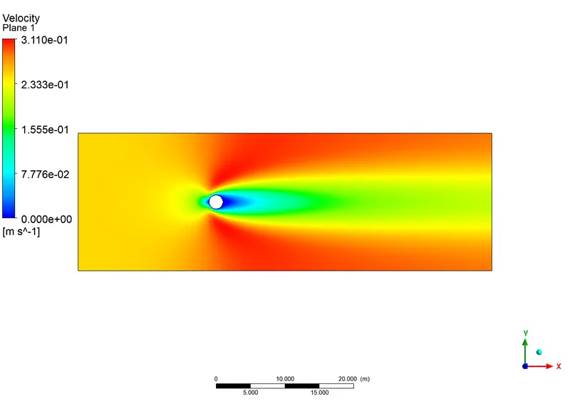
Reynold's number: 10
Flow velocity: 0.25`m/s`
viscocity: 0.05`(kg)/(m*s)`
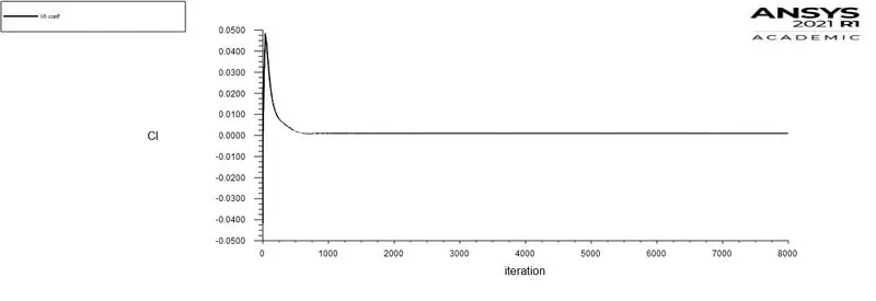
Residual Plot:
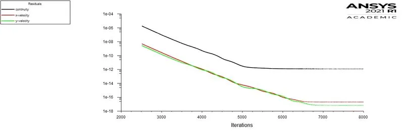
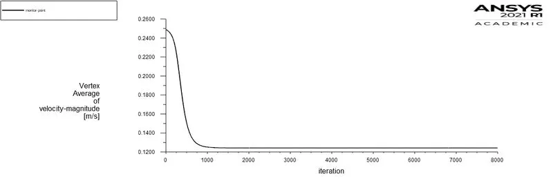
Monitor point velocity:
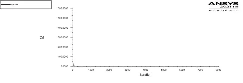
Plot of coefficient of drag:
Plot of coefficient of lift:
Velocity contour:
2. case-2
Reynold's number: 100
Flow velocity: 2.5`m/s`
viscocity: 0.05`(kg)/(m*s)`
Residual Plot:
Monitor point velocity:
Plot of coefficient of drag:
Plot of coefficient of lift:
Velocity contour:
3. case-3
Reynold's number: 1000
Flow velocity: 25`m/s`
viscocity: 0.05`(kg)/(m*s)`
Residual Plot:
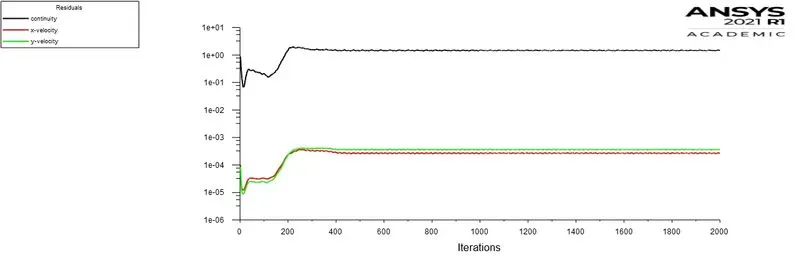
Monitor point velocity:
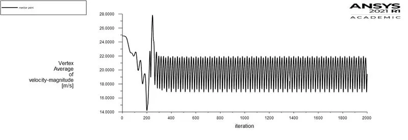
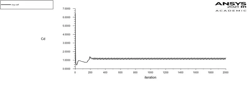
Plot of coefficient of drag:
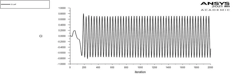
Plot of coefficient of lift:
Velocity contour:
4. case-4
Reynold's number: 10000
Flow velocity: 250`m/s`
viscocity: 0.05`(kg)/(m*s)`
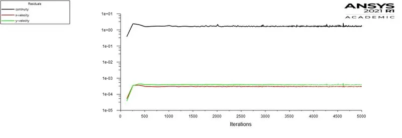
Residual Plot:
Monitor point velocity:
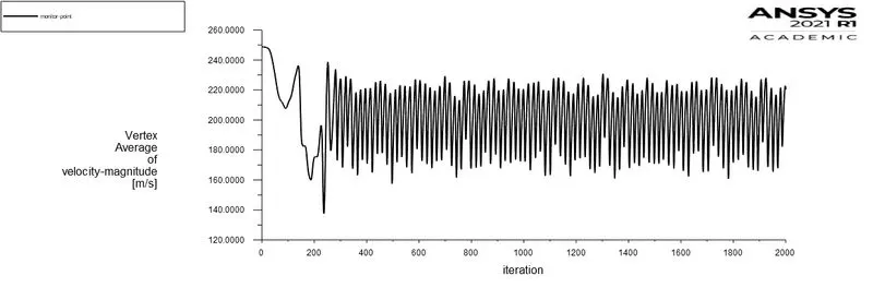
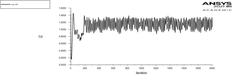
Plot of coefficient of drag:
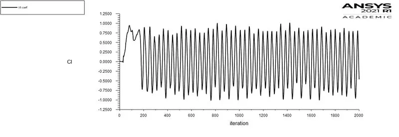
Plot of coefficient of lift:
Velocity contour:
6. case-6
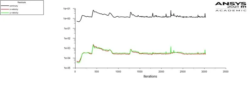
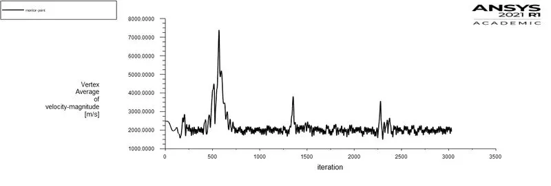
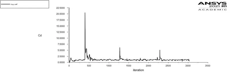
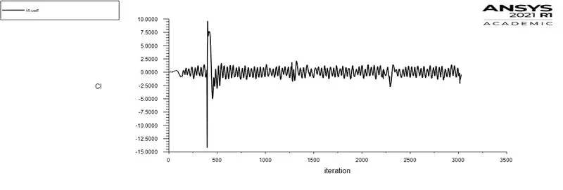
Reynold's number: 100000
Flow velocity: 2500`m/s`
viscocity: 0.05`(kg)/(m*s)`
Residual Plot:
Monitor point velocity:
Plot of coefficient of drag:
Plot of coefficient of lift:
Velocity contour:
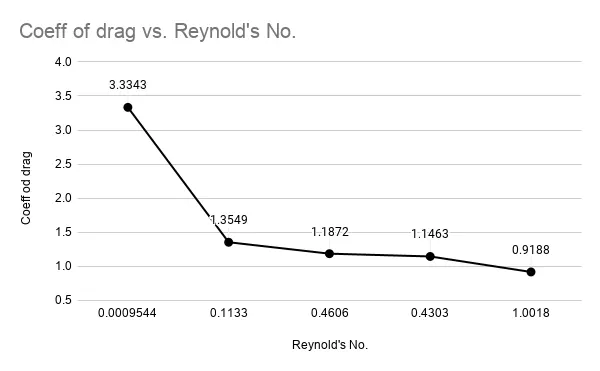
Comparison of Coeff of drag with Reynold's number:
| Reynold's No. | Coeff of lift | Coeff of drag |
| 10 | 0.0009544 | 3.3343 |
| 100 | 0.1133 | 1.3549 |
| 1000 | 0.4606 | 1.1872 |
| 10000 | 0.4303 | 1.1463 |
| 100000 | 1.0018 | 0.9188 |
Conclusion:
When Re increases it can be seen that the coefficient of drag increases. Between Re = 10 and Re = 50 that wake grows into a recognizable “wake” consisting of, recirculating eddy. Thus when Re>10000 turbulent eddies starts to form which ditatches and move along the flow and thus create a varying lift with a frequency. This can be inter pretted from the grtaph of coefficient of lift where the cylinder faces lift in a periodical manner in both direction also the monitor point velocity also shows a constantly varing velocity having a particular frequency.