Week 2 - Flow over a Cylinder.

Aim :

Simulate the flow over a cylinder and explain the phenomenon of Karman vortex street.

PART-I

1. Simulate the flow with the steady and unsteady case and calculate the Strouhal Number for Re= 100.

PART-II

1. Calculate the coefficient of drag and lift over a cylinder by setting the Reynolds number to 10,100,1000,10000 & 100000. (Run with steady solver)
2. Discuss the effect of Reynolds number on the coefficient of drag. [ Results should be validated with any standard literature and error should be within 5 %]

Objectives :

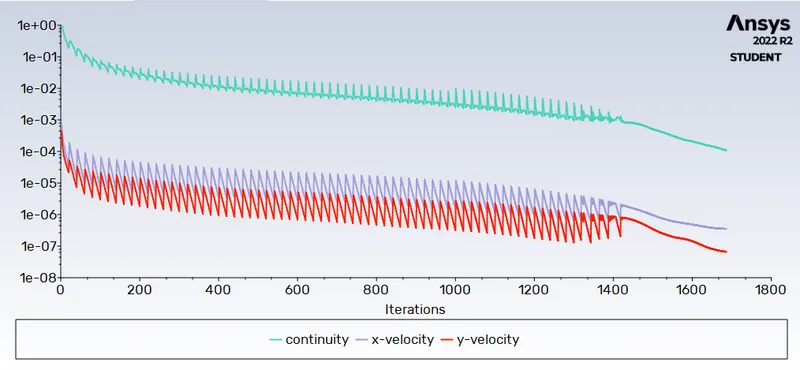
1. In both approaches, show that the flow has converged. That is, what quantities or plots need to be looked at to determine that the flow has converged?
2. Plots of the coefficient of drag and lift.
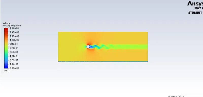
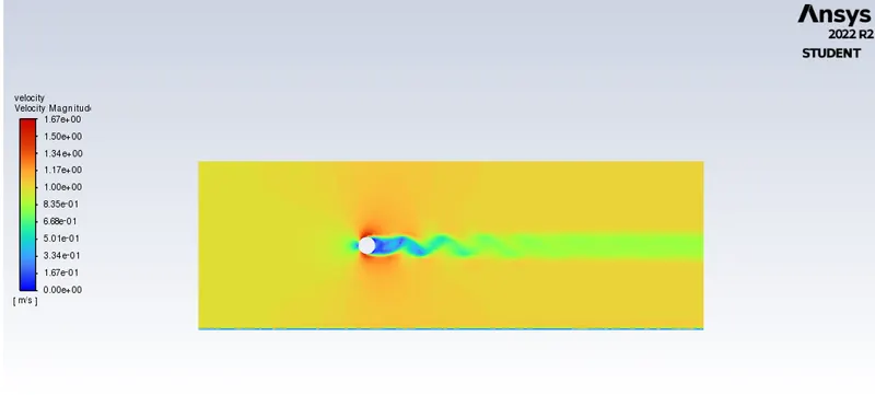
3. Plots to show vortex shedding behind the cylinder.
4. Mention the referred material (Reference Paper or Fluid Mechanics Textbook) at the end of the challenge submission page.

Theory :

In fluid dynamics, a Kármán vortex street is a repeating pattern of swirling vortices, caused by a process known as vortex shedding, which is responsible for the unsteady separation of flow of a fluid around blunt bodies.

It is named after the engineer and fluid dynamicist Theodore von Kármán and is responsible for such phenomena as the "singing" of suspended telephone or power lines and the vibration of a car antenna at certain speeds. Mathematical modeling of von Kármán vortex street can be performed using different techniques including but not limited to solving the full Navier-Stokes equations with k-epsilon, SST, k-omega and Reynolds stress, and large eddy simulation (LES) turbulence models, or by numerically solving some dynamic equations such as the Ginzburg-Landau equation

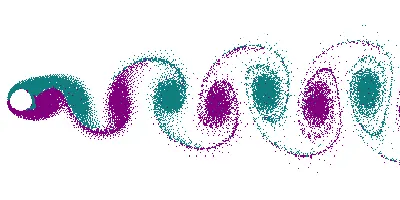
A vortex street will form only at a certain range of flow velocities, specified by a range of Reynolds numbers (Re), typically above a limiting Re value of about 90. The (global) Reynolds number for a flow is a measure of the ratio of inertial to viscous forces in the flow of a fluid around a body or in a channel, and may be defined as a nondimensional parameter of the global speed of the whole fluid flow:

where:

• = the free stream flow speed (i.e. the flow speed far from the fluid boundaries like the body speed relative to the fluid at rest, or an inviscid flow speed, computed through the Bernoulli equation), which is the original global flow parameter, i.e. the target to be non-dimensionalised.
• = a characteristic length parameter of the body or channel
• = the free stream kinematic viscosity parameter of the fluid, which in turn is the ratio:

Where,

• = the reference fluid density.
• = the free stream fluid dynamic viscosity

Solution :

1. Geometry :

The following are the tools we used to create the geometry and we have the same after the attempt of creation.

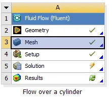
Create geometry in space claim

We used line tool to draw with dimensions :

cylinder dia - 2m, with circle origin - -20 on X and +40 on X-axis.

box - 60x20m

and then used Pull to create a surface from the geometry that looks like

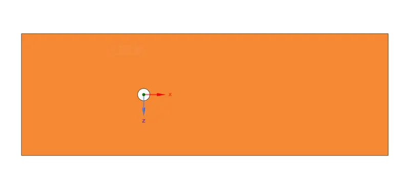
Close the geometry and open mesh

2. Meshing :

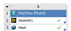
next update the geometry and open mesh.

Here we are going to perform mesh and to achieve a very fine Triangular mesh we have to perform certain steps to make sure it is desirable and

we are to be some different methods and tools to do so. Below are the steps involved in order to do so. This is the former mesh.

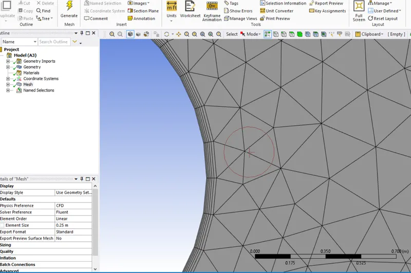
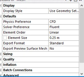
name the section as below :

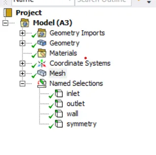
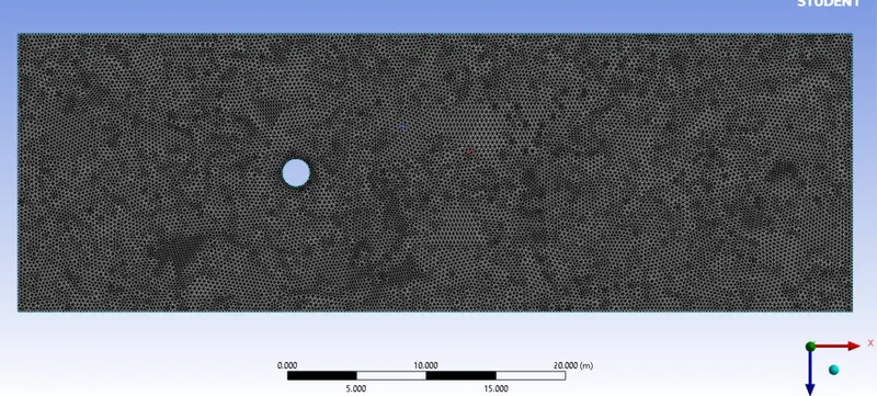
As we can see the layers are formed as we provided the layer quantity to the wall edge and that's how we get the finer edge mesh.

3. setup :

PART-I

1. Simulate the flow with the steady and unsteady case and calculate the Strouhal Number for Re= 100.

Moving on to the Fluent we will simulate the above mesh with steady-state simulation and calculate the strouhal number. This part has 2 cases so first we run simulation for steady state. We will also animate the following output and to plot the contour.

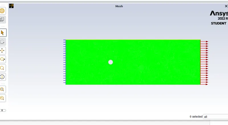
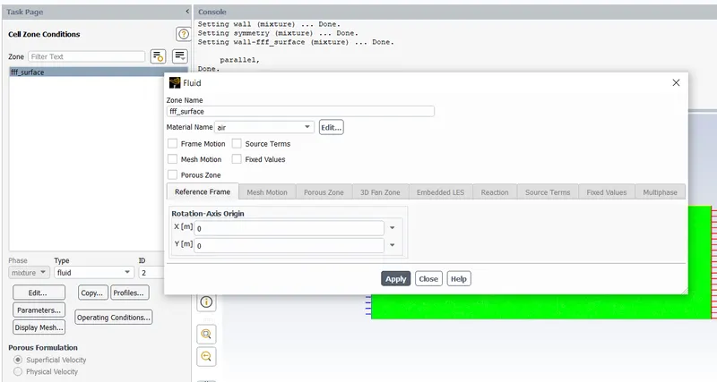
Giving cell zone conditions :

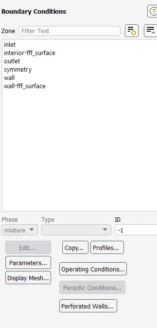
Giving boundary Conditions :

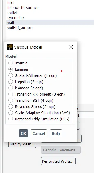
Select laminar flow

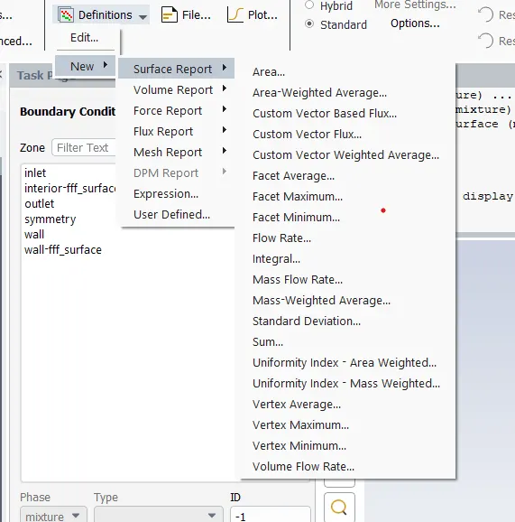
Defining surface reports :

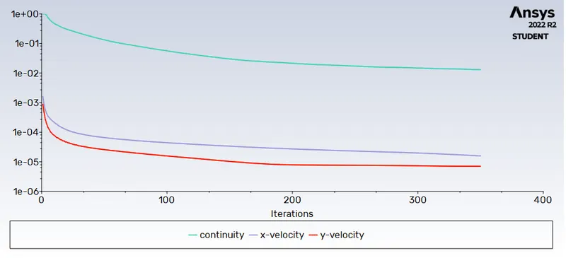
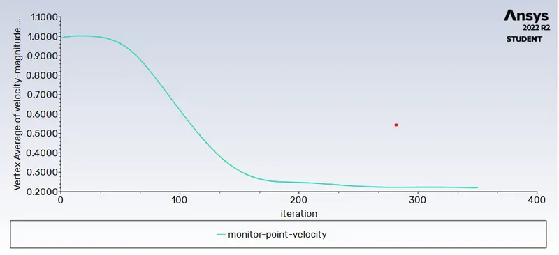
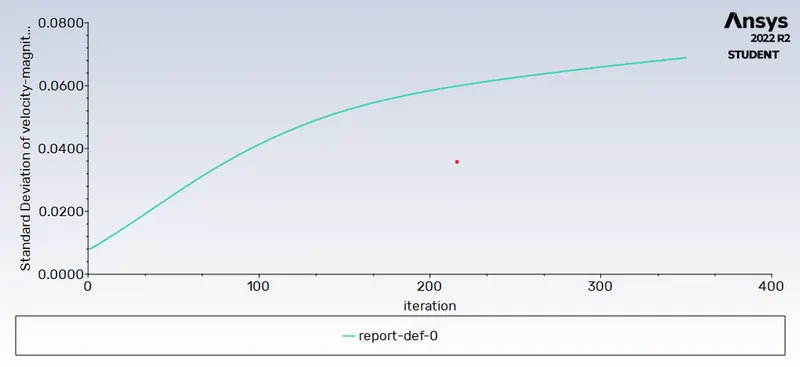
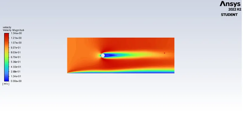
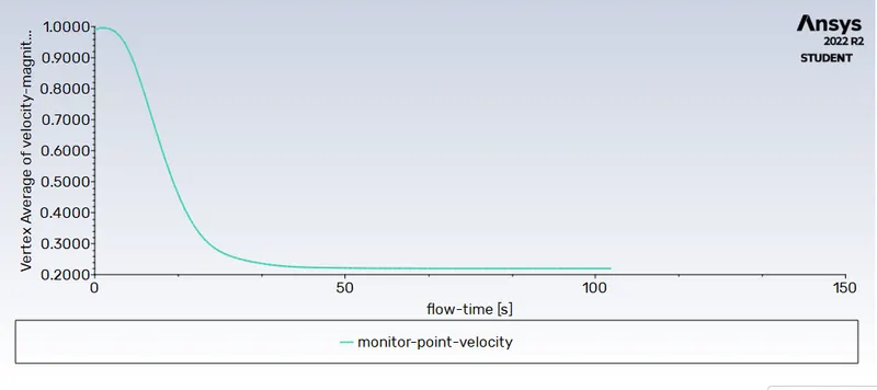
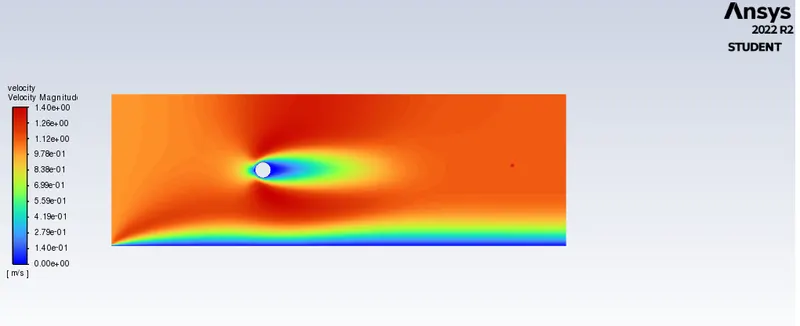
Case 2: Steady state simulation of reynolds number 100.

Monitor point velocity :

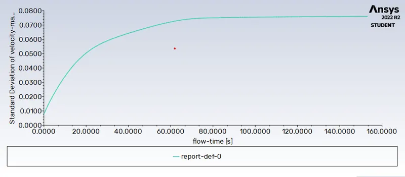
Standard deviation :

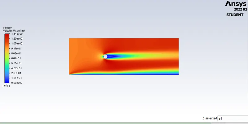
The contour of velocity magnitude :

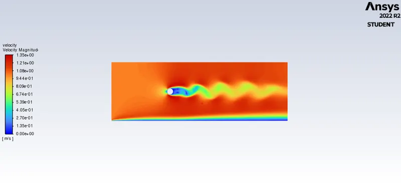
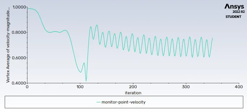
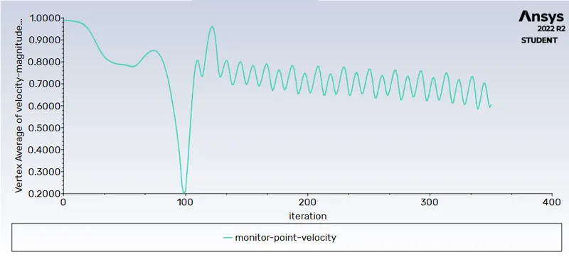
case 2 : Transient state simulation of Reynolds number 100.

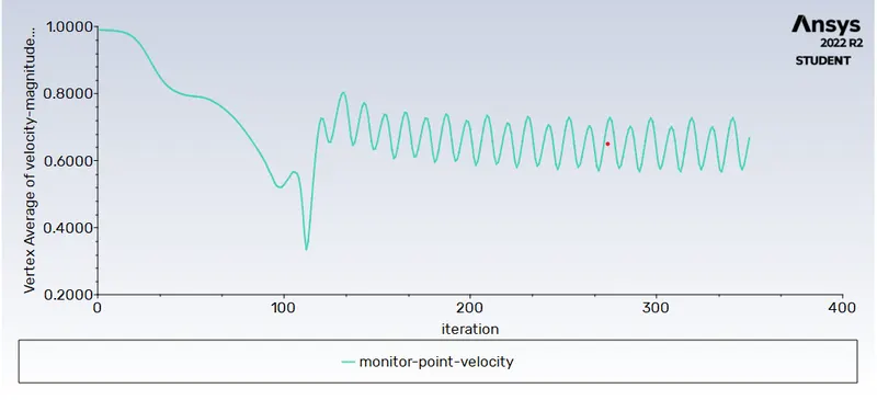
Monitor point velocity :

Standard deviation :

The contour of velocity magnitude :

Video link :

https://youtu.be/1v-038pJC9M

PART-II

1. Calculate the coefficient of drag and lift over a cylinder by setting the Reynolds number to 10,100,1000,10000 & 100000. (Run with steady solver)
2. Discuss the effect of Reynolds number on the coefficient of drag. [ Results should be validated with any standard literature and error should be within 5 %]

Solution 1:

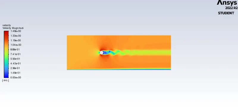
As we move forward for calculating the coefficient of drag and lift with Reynolds number. All the steps are the same as running the case in Fluent where we have to change the viscosity value in materials with different values and run the case.

Reynolds number : 10 100 1000 10000 100000

Viscosity : 0.2 0.02 0.002 0.0002 0.00002

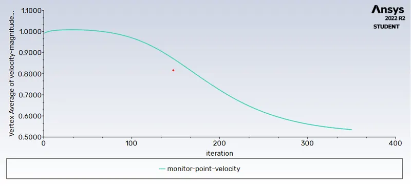
with viscosity 0.2

with viscosity 0.02

with viscosity 0.002

with viscosity 0.0002

with viscosity 0.00002

Solution 2:

The effect of Reynolds number on the coefficient of drag and Lift done by aerodynamic experimentation of an airfoil with gurney flap

Lift coefficient decreases rapidly and drag coefficient increases rapidly when Reynolds number is decreased below critical range. This occurs due to a change in flow pattern near the Gurney flap at low Reynolds numbers.

• Reynolds number plays a very major role in the airfoil aerodynamics for the NACA0012 airfoil without and with Gurney flap. Lift decreases and drag increases when Reynolds number is decreased.
• For the airfoil with GF, Reynolds number has adverse effects on lift coefficient, while the drag coefficient of the airfoil with GF has some beneficial effects compared to the airfoil without GF.
• For high Reynolds number above critical range, decrease in Cl and Cd increase in are negligible.
• As the Reynolds number is decreased below the critical Reynolds number range, Cl decreases and Cd increases at a very steep rate and the performance degrade rapidly.
• For lower Reynolds numbers, the two vortices behind the Gurney flap vanish. The Gurney flap seems to increase the effective camber of the airfoil, causing a negative zero-lift angle and reduced stall angle.

Conclusion of both cases:

And In both approaches, the flow has converged and we looked at a monitored control point plot to make sure that estimation. The frequent curve frequency shows that there's the presence of a physical phenomenon of vortex shedding around the cylinder wall.