Week 2 - Flow over a Cylinder.
Objective:
Simulate the flow over a cylinder and explain the phenomenon of Karman vortex street.
PART 1:
Simulate the flow with the steady and unsteady case and calculate the Strouhal Number for Re= 100.
PART-II
- Calculate the coefficient of drag and lift over a cylinder by setting the Reynolds number to 10,100,1000,10000 & 100000.
- Effect of Reynolds number on the coefficient of drag. [ Results should be validated with any standard literature and error should be within 5 %]
Introduction:
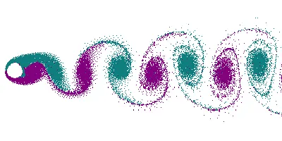
Vortex shedding is an oscillating flow that takes place when a fluid such as air or water flows past a bluff (as opposed to streamlined) body at certain velocities, depending on the size and shape of the body. In this flow, Vortices are created at the back of the body and detach periodically from either side of the body, forming a von Karman vortex street. The fluid flow past the object creates alternating low-pressure vortices on the downstream side of the object. The object will tend to move toward the low-pressure zone. Moreover, von Kármán vortex street is a repeating pattern of swirling vortices, caused by a process known as vortex shedding, which is responsible for the unsteady separation of flow of a fluid around blunt bodies.In flow past a cylinder this vortex can be seen at onset of RE=40 and upto RE=400.About reynold no 200 this vortex street becomes three-dimensional.
Strouhal Number:
The Strouhal number is a dimensionless number describing oscillating flow mechanisms
The Strouhal number is often given as

where f is the frequency of vortex shedding
L is the characteristic length
U is the flow velocity
A brief explanation to solve the flow over a cylinder
Procedure
Geometry:
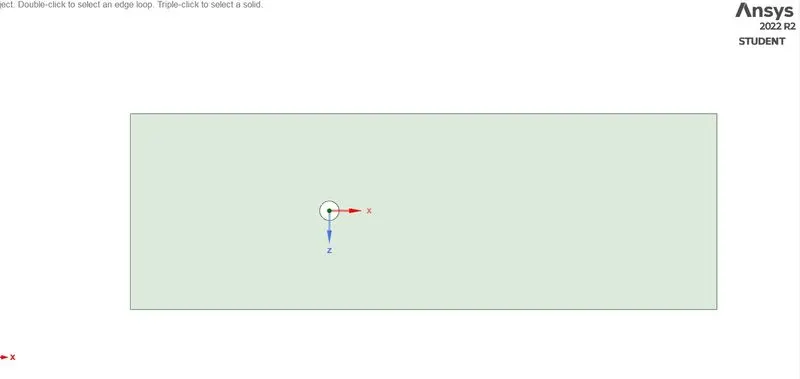
Creating the geometry by sketching using the line and circle command, circle diameter of 2m and the dimensions having 20X60m and the circle is placed 20m from the inlet. Converting the geometry into the surface by using command pull and select. Also, delete the inside the circle to carry out the simulation.
Mesh:
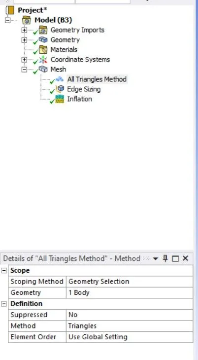
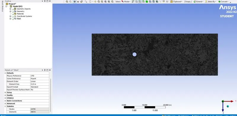
First of all, the baseline mesh autogenerated quad mesh was created. After that, it will change according to simulation requirements, and it was finely tuned with the help of triangular mesh generated. The model meshed with an element size of 0.23m.
Edge sizing:
Body fitted mesh is generated.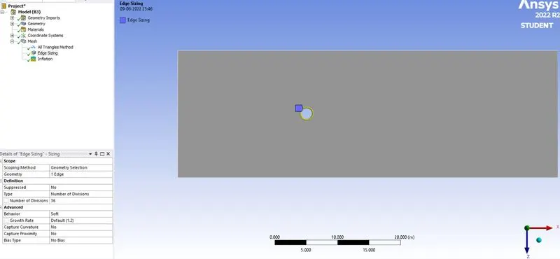
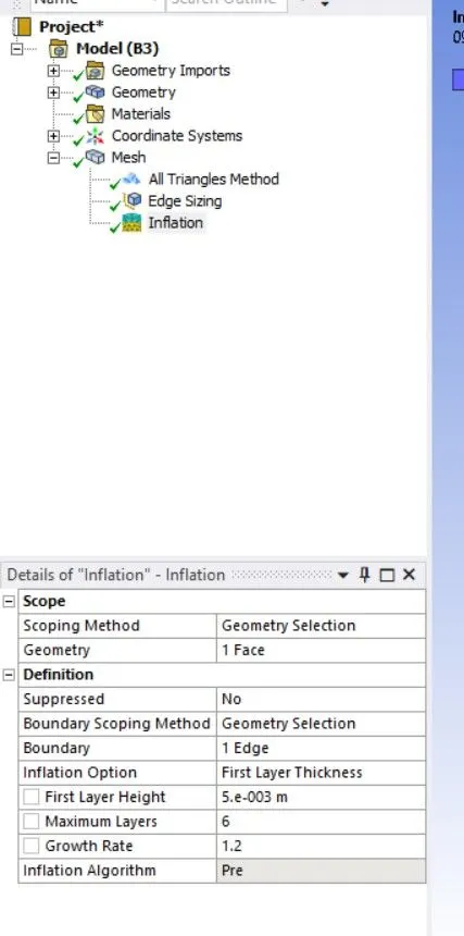
Inflation layer:
To capture the better results near the cylinder wall inflation layer set up is used.
Boundary flagging:
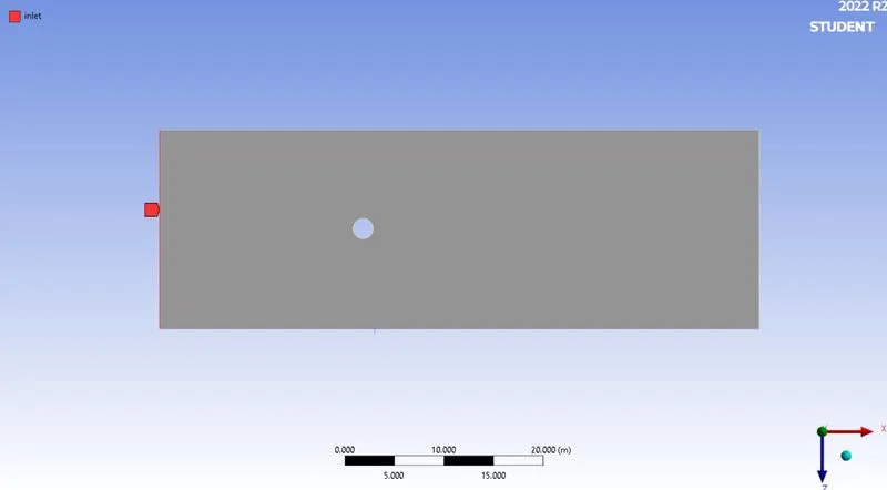
Inlet:
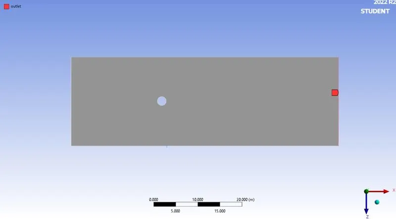
Outlet:
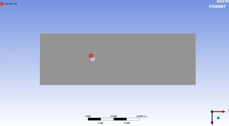
Cylinder Wall:
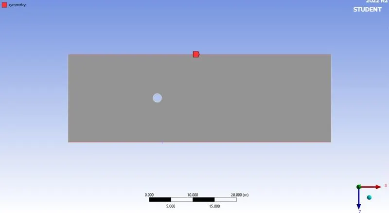
Symmetry:
Setting up physics, boundary conditions and output:
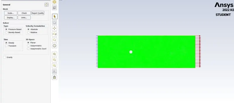
For steady state:
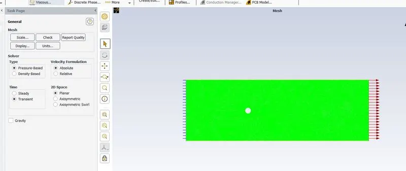
Unsteady state:
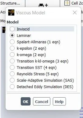
Viscous Model:
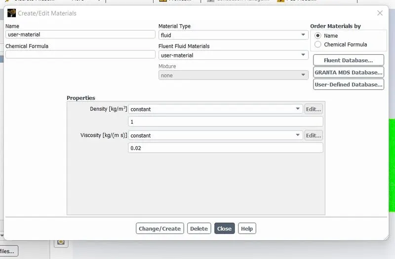
Material:
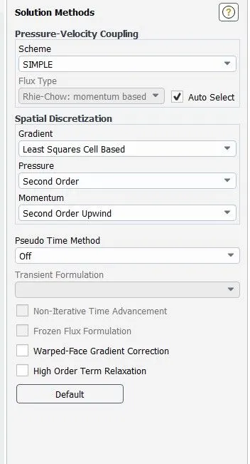
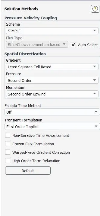
Solving method ( Steady and Unsteady state ):
For velocity-pressure coupling, the SIMPLEC algorithm was used. When the SIMPLEC algorithm is used, the pressure under-relaxation is automatically increased to 1.0. The setting for pressure under-relaxation is 0.3 (when the default SIMPLE algorithm is used). Here the momentum under-relaxation has also been increased from 0.7 to 0.9 to yield better convergence.
Steady state:
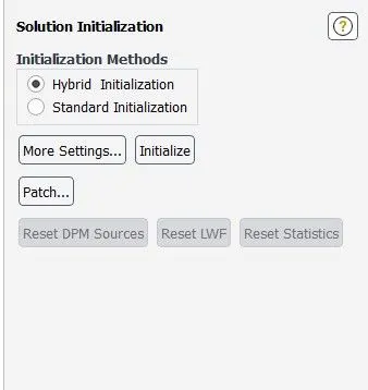
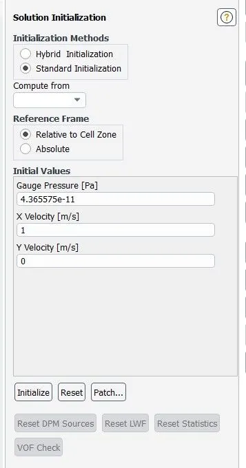
Solution initialization :
Unsteady state:
Solution initialization :
steady-State Simulation:
The following plots to be shown for both steady and unsteady simulation
Plots:
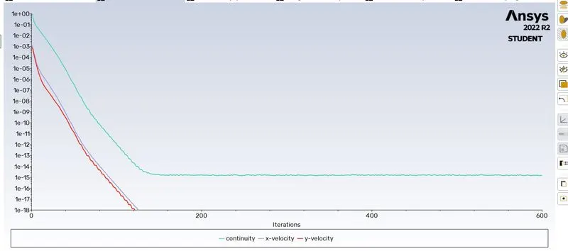
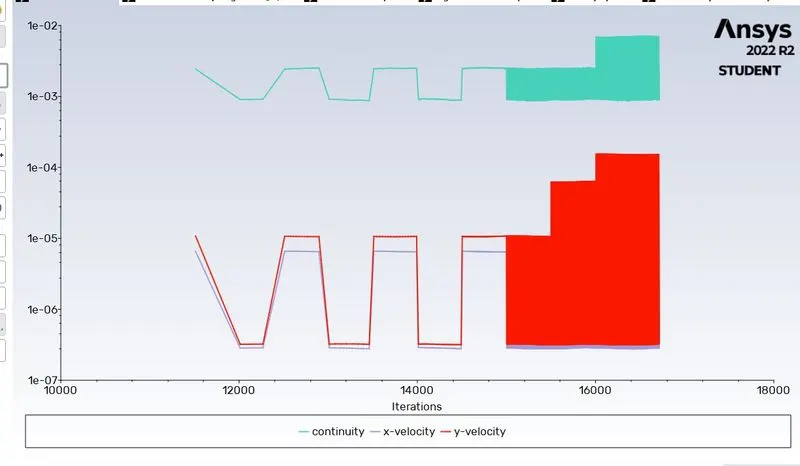
Residual plot:
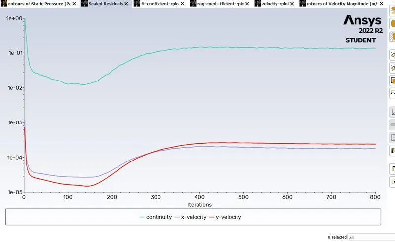
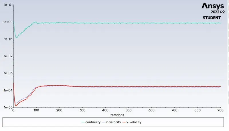
This plot shows at what point convergence has achieved.
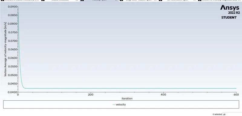
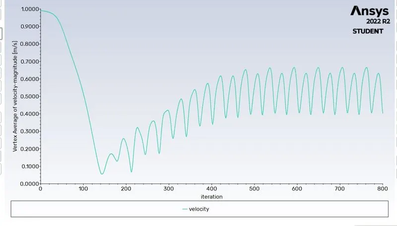
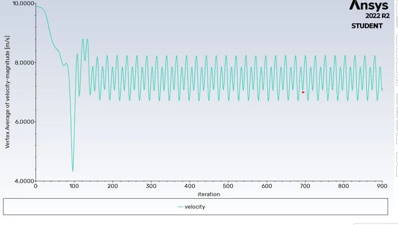
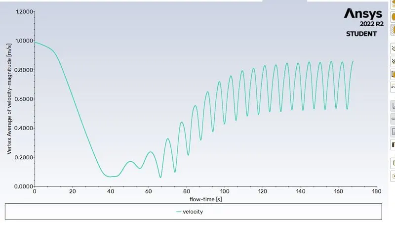
Monitor point velocity plot:
The monitor of 8m is placed at a distance from the cylinder to calculate the velocity from that point.
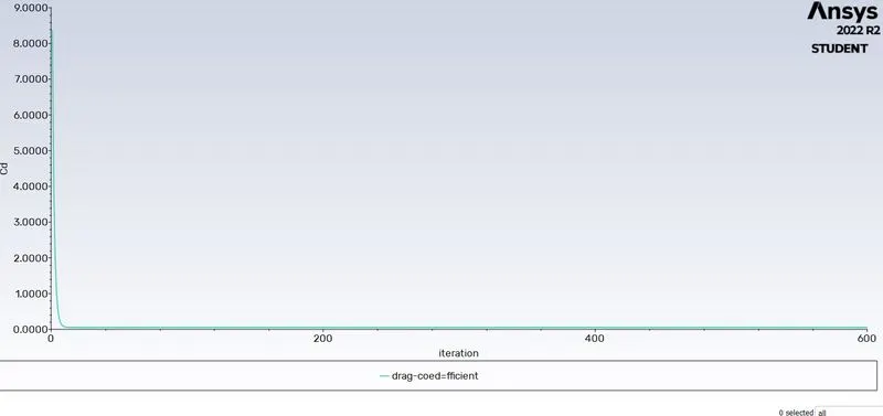
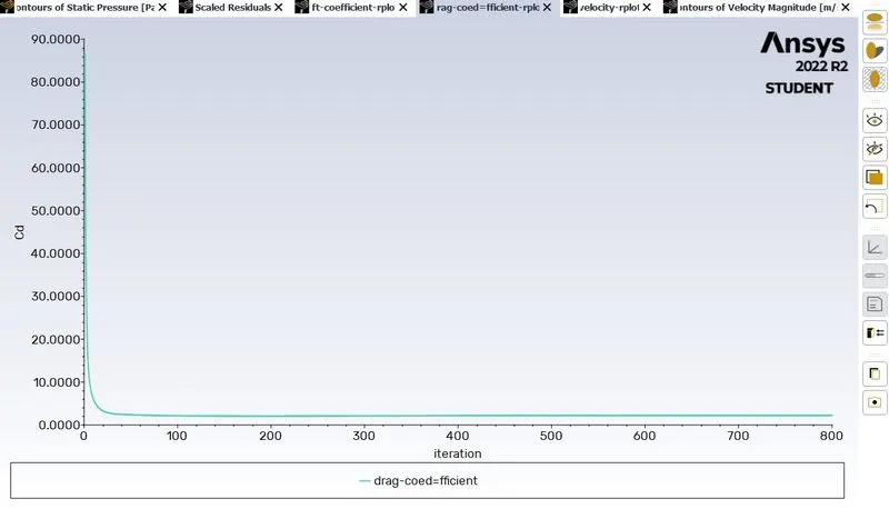
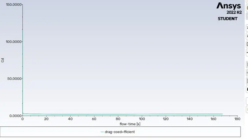
Drag Coefficient Plot:
To calculate the drag coefficient.
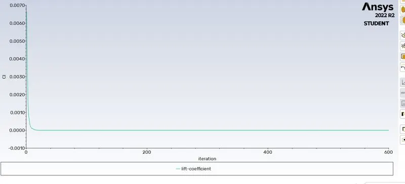
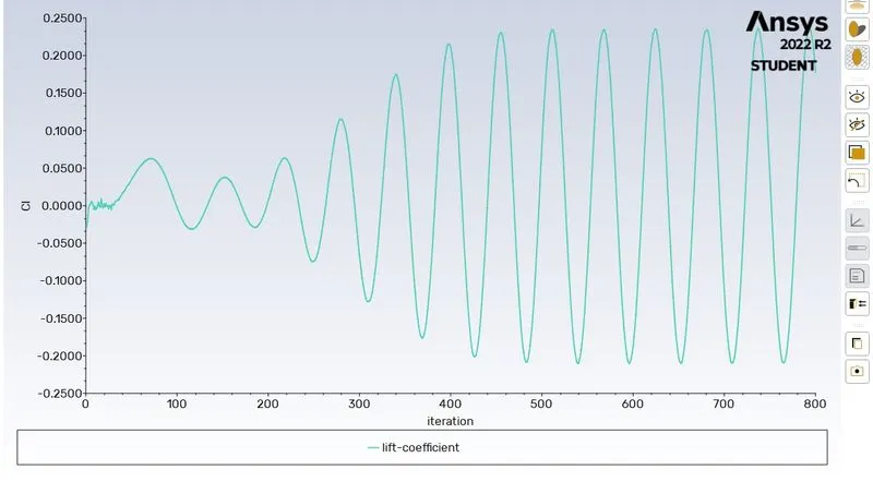
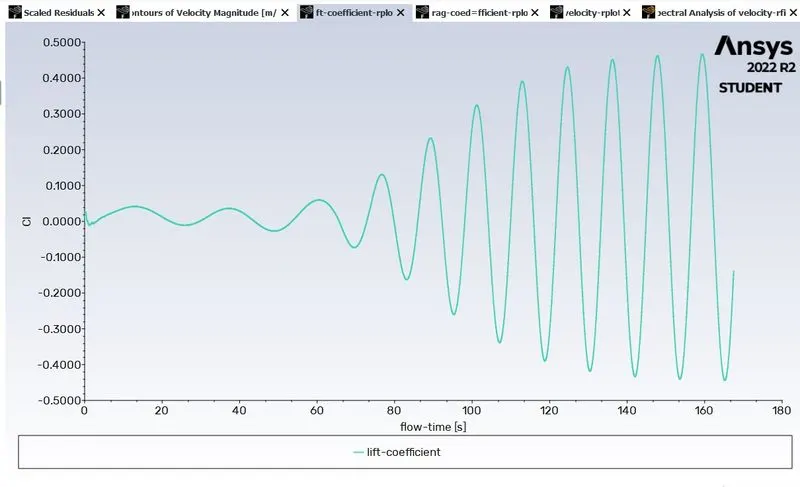
Lift Coefficient Plot:
To calculate the lift coefficient.
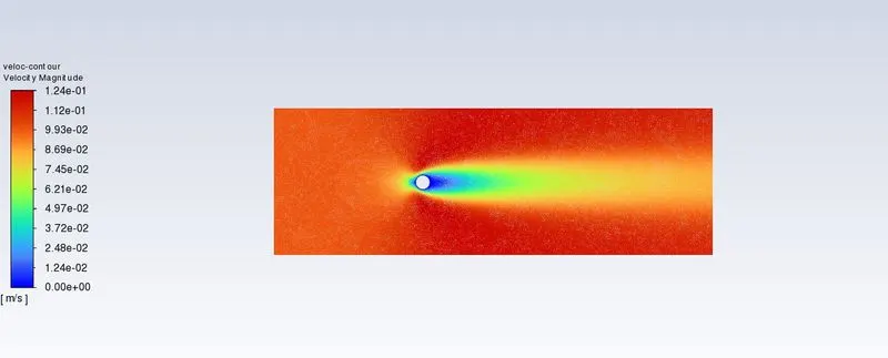
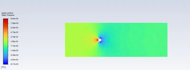
Velocity & Pressure Contour:
To see the velocity & pressure changes when flow past over a cylinder.
Case 1:
Reynolds Number = 10
viscosity = 0.02
Velocity = 0.1
Iterations = 600
Residual plot:
Monitor point velocity:
Drag Coefficient:
Lift coefficient:
Velocity contour:
Pressure contour:
https://drive.google.com/file/d/1XWv9QXx1Gm5PLOX-E8qIH5ohoT66slrN/view?usp=sharing
Case 2 :
Reynolds number: 100
velocity: 1
viscosity: 0.02
Iterations: 800
Residual plot:
Monitor point velocity:
Drag Coefficient:
Lift coefficient:
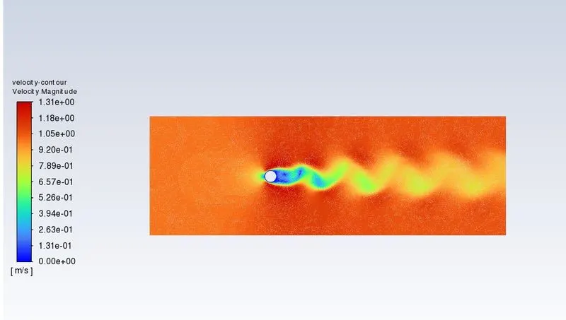
Velocity contour:
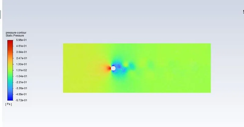
Pressure contour:
Video animation:
https://drive.google.com/file/d/1HLYuszIeJ7bTy9p0UxzTcQV9dfhPJ0i9/view?usp=sharing
Case 3:
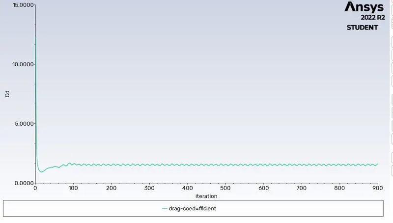
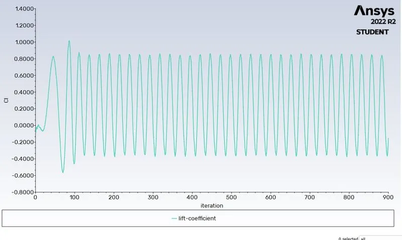
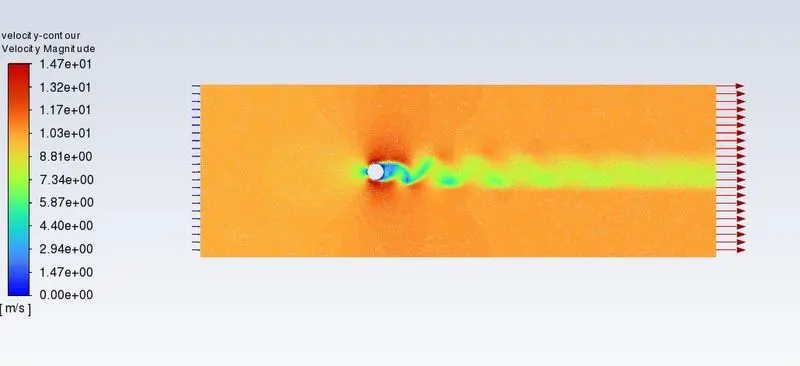
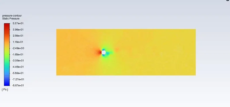
Reynolds number: 1000
Velocity: 10
viscosity : 0.02
Iterations: 900
Residual plot:
Monitor point velocity:
Drag Coefficient:
Lift coefficient:
Velocity contour:
Pressure contour:
Video animation:
https://drive.google.com/file/d/1wKbbAhWF5rrG50dn1ehGH1p4VxaYME5z/view?usp=sharing
Case 4:
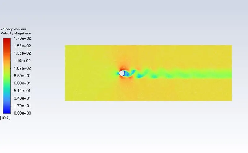
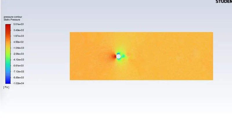
Reynolds Number: 10000
Viscosity: 0.02
Velocity: 100
Iterations: 1100
Residual plot:
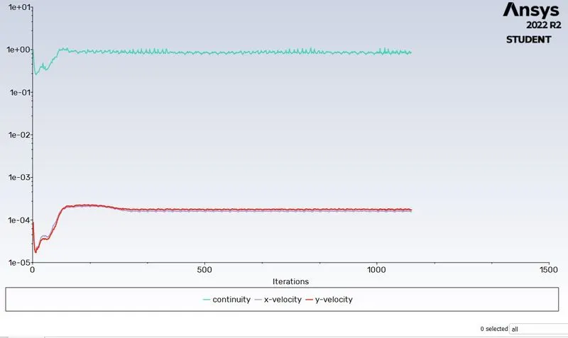
Monitor point velocity:
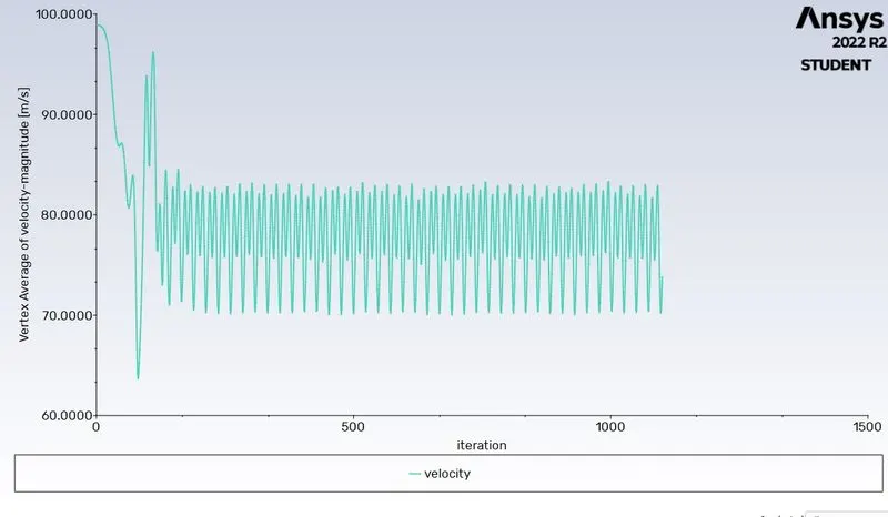
Drag Coefficient:
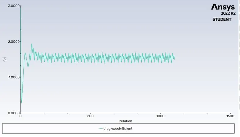
Lift coefficient: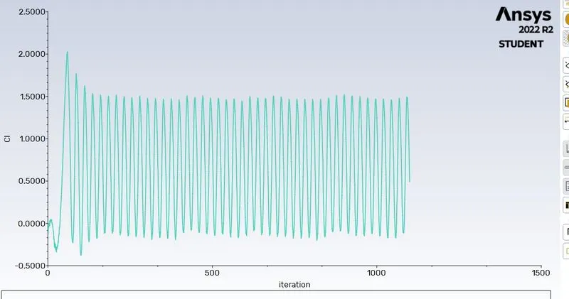
Velocity contour:
Pressure contour:
Video animation :
https://drive.google.com/file/d/1-CeDl80QlZr5o09q8i-bUlBm6QtKpy8y/view?usp=sharing
Case 5:
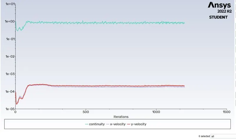
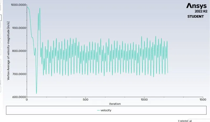
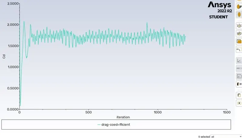
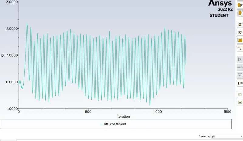
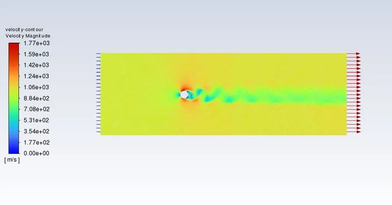
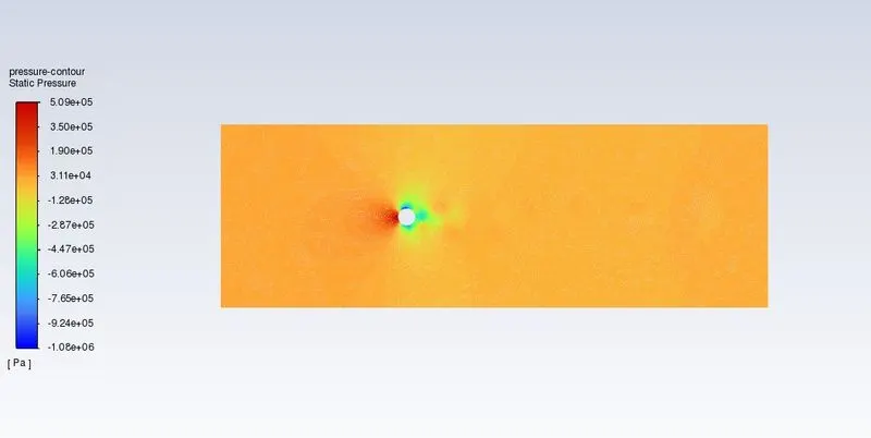
Reynolds Number: 100000
Viscosity:0.02
Velocity:1000
Iterations:1200
Residual plot:
Monitor point velocity:
Drag Coefficient:
Lift coefficient:
Velocity contour:
Pressure contour:
https://drive.google.com/file/d/1jCIFR5774IKNpvLuMsUOBcsRdVB0e5mL/view?usp=sharing
Unsteady State:
Reynolds Number: 100
Viscosity:0.02
Velocity:1
Iterations: 16750
Time step: 0.05
Residual plot:
Monitor point velocity:
Drag Coefficient:
Lift coefficient:
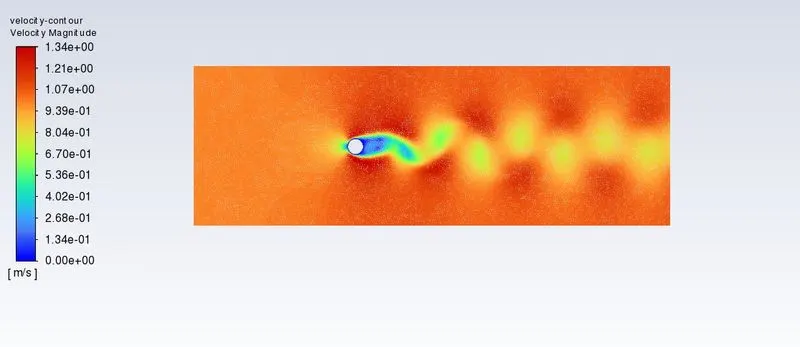
Velocity contour:
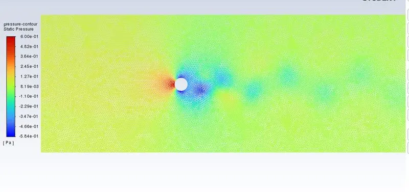
Pressure contour:
Strouhal Number calculation:
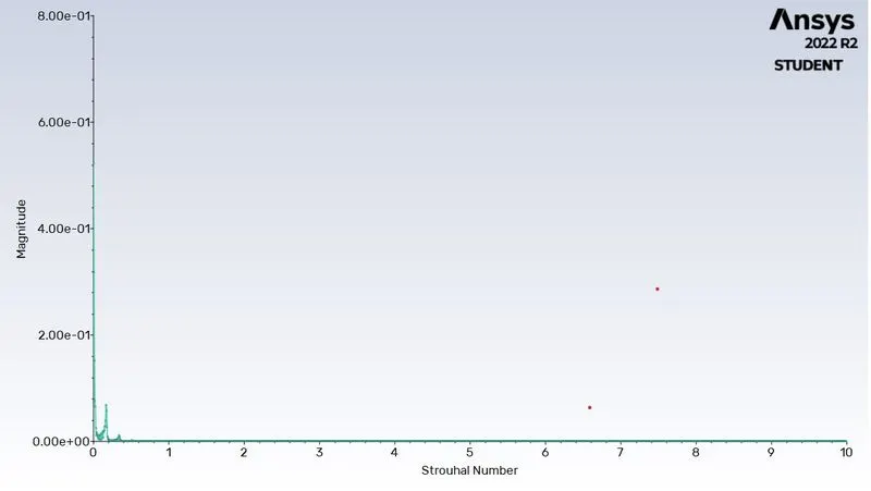
At maximum magnitude the value of f from graph=0.08162
Strouhal Number = (f*D) /v = (0.08162 * 2)/ 1
= 0.1632
Animation video
https://drive.google.com/file/d/1jhgOpnvIvN-Rj66kvEJ_MUdGlUWJDqTN/view?usp=sharing
| Reynolds Number | Coeffecient of drag | coeffecient of lift |
| 10 (Steady State) | 2.664 | 0.00173 |
| 100 (Steady State) | 2.2324 | 0.17382 |
| 100 (Unsteady State) | 2.288 | 0.0798 |
| 1000 (Steady State) | 1.5943 | 0.1494 |
| 10000 (Steady State) | 1.4996 | 0.481277 |
| 100000 (Steady State) | 1.7184 | 0.653152 |
Conclusion:
When the reynolds number increases the coeffecient of drag decreases. Moreover, when the reynolds number is large (Re>4000) flow will be turbulent( Chaotic and swirling vortices), in which laminar flow is very small and which leads to lower skin friction drag.
Firstly , when the velocity increases coeffecient of drag decreases.
Secondly, for the reynolds number 10 no vortices can be seen because of low velocity and only boundary layer seperation occured.Also, in low reynolds number coeffecient of drag increases.
For reynolds number 100 ( Unsteady state) the vortices can be seen and the shedding frequency calculated.In addition, the value of 0.16 strouhal number is calculated.We have validated this result with experimental data (0.165) were the error appears to be less than 5%.
In this case the blundary layer seperation decreases there will be less recirculation flow at wake region behind the cylinder with the reduced drag.For all the simulation parameters are kept constant except for the velocity, so increasing the velocity will increase reynolds number.
For the steady case the flow is not dependent on time step so strouhal number cannot be calculated for the steady state but the solution has reached the steady state after some iterations. We can seen vortices for higher reynolds number only.
For better visualization we can use contour, vector and streamline to see the vortex generation when the flow past over a cylinder.
In transient case lift coeffecient keeps on changing beacuse of alternate nature of the vortices it never settle down and keeps on repeating same pattern after some iteration( residual plot).When it comes to steady case the flow is not dependent time so the lift coeffecient becomes constant after some iterations.
Preferred material for instability:
In order to prevent the unwanted vibration of cylindrical bodies, a longitudinal fin can be fitted on the downstream side, which, provided it is longer than the diameter of the cylinder, will prevent the eddies from interacting, and consequently they remain attached. Obviously, for a tall building , the relative wind could come from any direction. For this reason, helical projections resembling large screw threads are sometimes placed at the top, thereby discouraging the alternate shedding of vortices. Another countermeasure with tall buildings is using variation in the diameter with height, such as tapering - that prevents the entire building being driven at the same frequency. For example, spiral added to the chimney to avoid vortex shredding