Week 2 - Flow over a Cylinder.

Aim:

• To simulate flow over a cylinder by using a 2D surface as model
• Differentiate among solving steady and unsteady solvers
• Calculate strouhal number
• Effect of reynolds number on co-efficient of drag

Introduction:

Flow over a cylinder:

To clearly understand the aerodynamics of different bodies in various applications like in aerospace, marine systems, and automobiles, power generation needs CFD simulations for a better and efficient design. The aerodynamic structures employed for these applications are an enlarged form of a cylinder, and the analysis of flow over a cylinder forms the base for these analyses.

In this analysis, a circle enclosed in a rectangle, corresponding to a circular cross-sectional cylinder in a fluid domain is sketched and is simulated for varying reynolds number. The phenomenon of vortex shedding is studied, along with the relation between reynolds number and co-efficient of drag. A similar case of steady vs transient case is also simulated at Reynolds number=100 and the strouhal number relation is also studied.

Vortex shedding:

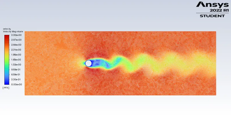
As known, the character of the incompressible steady flow of a classical fluid past an onstacle is determined by a single dimensionless parameter called the Reynolds number. For reynolds number less than 1, the flow is laminar. At Re~10, a pair of eddies appears behind the cylinder, and at Re~100 these eddies start to be cast off from the cylinder and is called the Karman vortex street formation.

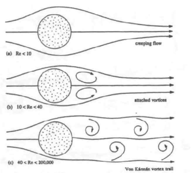
Further increase in reynolds number leads gradually to a region of fully-developed turbulence in the wake of the cylinder. There are two contributions to this physically phenomenon, the viscous force and a bernoulli acting opposite to it. As long as the bernoulli force is much less than the viscous force, the effect is negligible.

The flow at high reynolds number can be divided into two regions, separated by a surface of separation. Inside the region at the rear of the cylinder bounded by the surface of separation, there is fully-developed turbulence, outside it the flow is approximately that of an ideal fluid except in a thin boundary layer close to the surface of the cylinder. The net drag force on the cylinder is of particular interest and its value is expressed in terms of a drag co-efficient called the Co-efficient of drag, expressed by `Cd=(2.Fd)/(rho u^2 A)`

Strouhal number:

It is a dimensionless number which describes the oscillating flow mechanism. It can be defined as the ratio between oscillations and mean speed.

Mathematically, Strouhal number = `(omega L )/ u`, where `omega`is the frequency, `L`is the characteristic length, and `u` is the flow velocity.

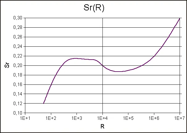
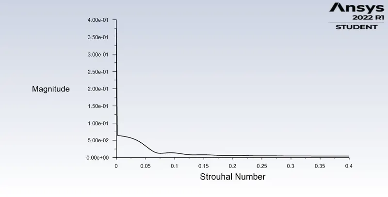
For a range of 0.1 to 0.3, the strouhal number greatly depends on the value of reynolds number. After that the strouhal number increases with increase in reynolds number. For low strouhal number (10e-4 or below), high speed steady state movement dominates the oscillation. The strouhal number can also be calculated for natural phenomenon like swimming of fish and flying of birds, characterised by a value between 0.2 to 0.4

Co-efficient of drag:

Procedure:

Step 1: Setting up geometry

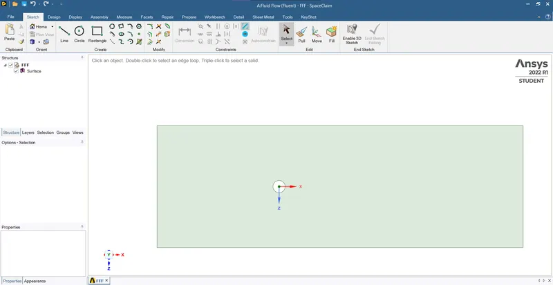
It is done in Space claim component.

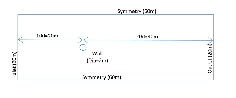
A 2D surface is sketched with a circle and a rectangle; the circle depicting the cross-section of a cylinder and rectangle depicting the domain to study.

Construction line tool is used to form the domain boundaries, circle and rectangle tool is used to draw the 2D sketch and pull tool is used to convert the 2D sketch into a surface.

Step 2: Meshing

Mesh component is updated with the geometry.

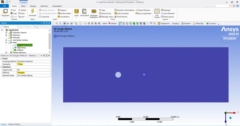
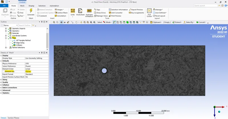
New method is inserted with triangle dominated mesh

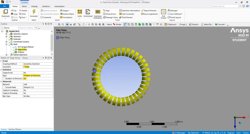
Edge sizing is done with 36 edges for the circle to preserve the shape of the object.

Inflation layers are added to create a body fitted mesh

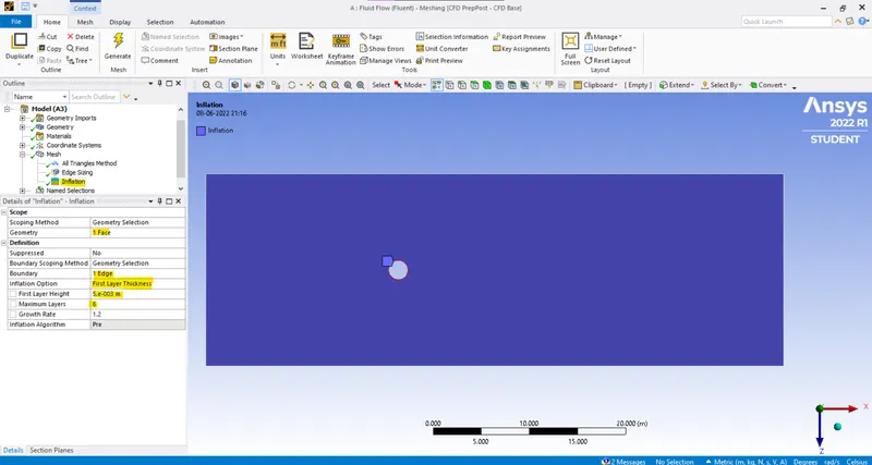
6 inflation layers with growth factor 1.2 is created

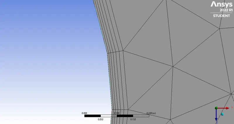
Generated mesh with element size 0.25m:

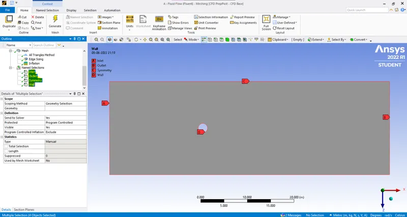
Boundaries are assigned to the geometry and mesh

Inlet, outlet, symmetry and wall are the types assigned

Step 3: Setting up domain and physics

Viscous model with laminar model is selected for the analysis

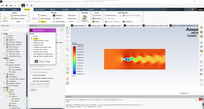
In laminar model, steady and transient state are used for analysis.

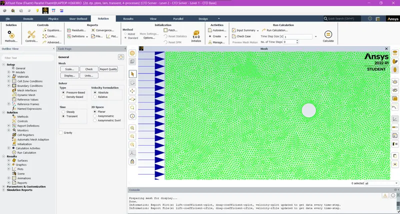
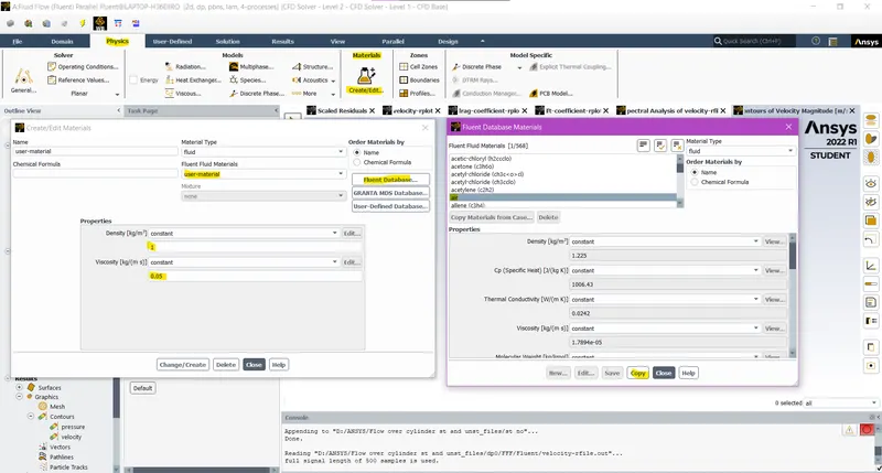
User material is defined by copying properties of air and defining density as 1 kg/m3 and viscosity as 0.05 kg-m/s, and is designated as the working fluid

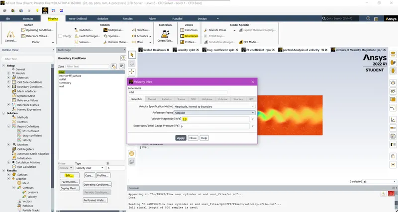
Boundary conditions for inlet, outlet, symmetry and wall are defined with inlet velocity as 2.5 m/s

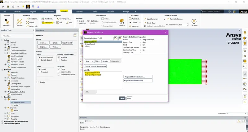
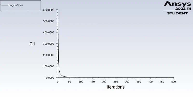
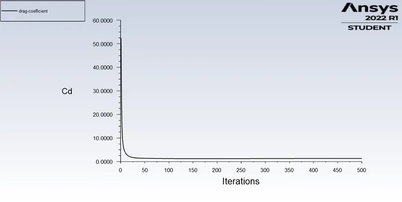
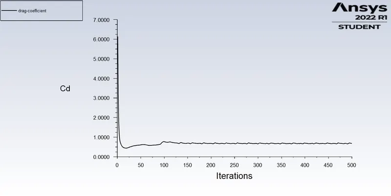
Surface plot criteria for drag co-efficient is set at wall edge

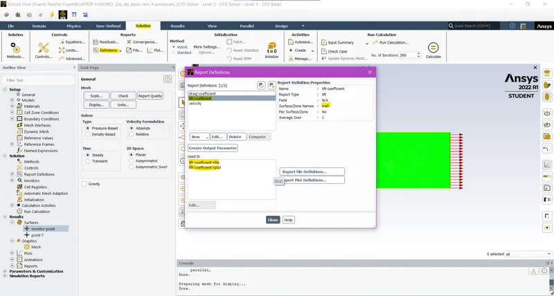
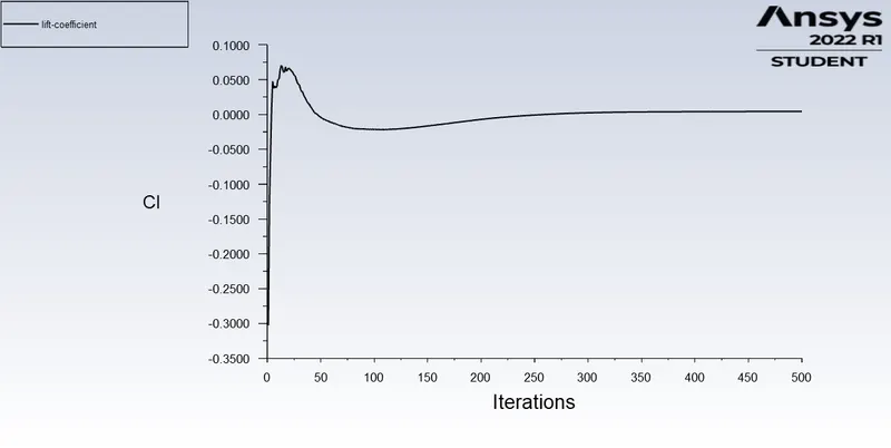
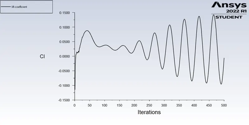
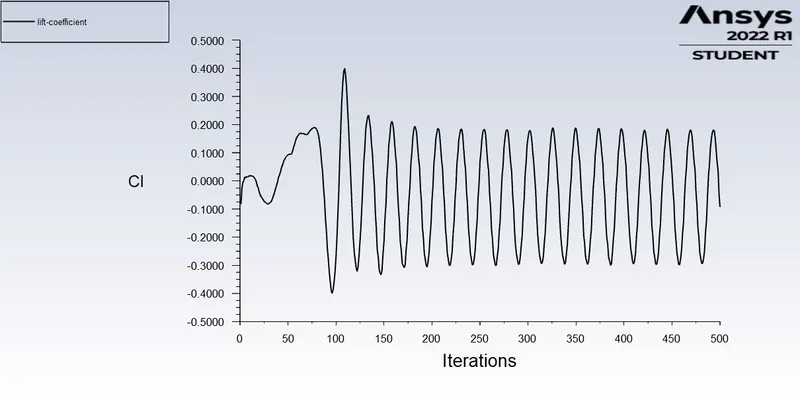
Surface plot criteria for lift co-efficient is set at wall edge

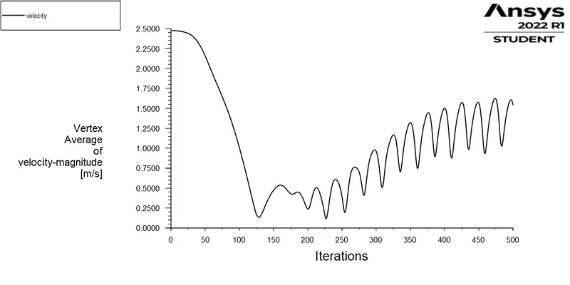
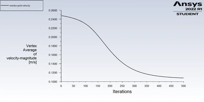
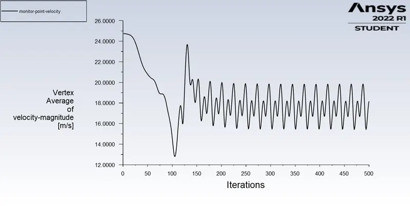
A monitor point on the surface is created to monitor velocity

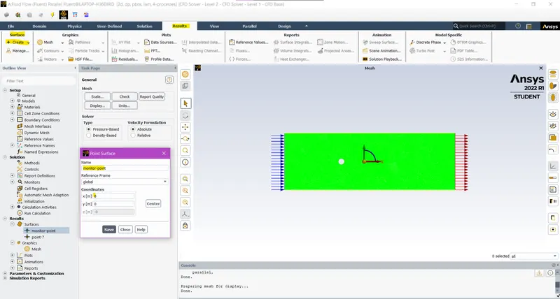
Surface plot criteria for velocity is set at the monitor point

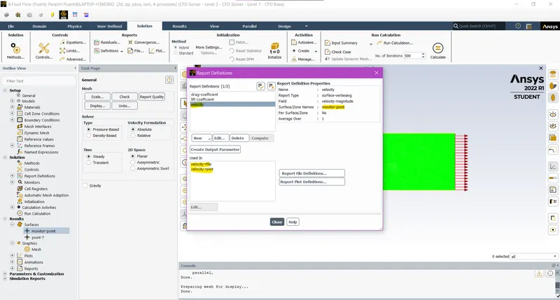
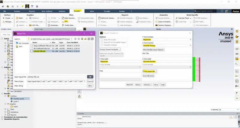
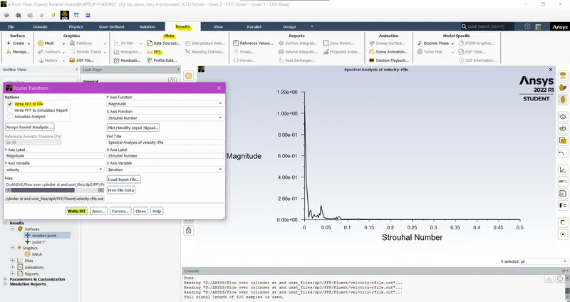
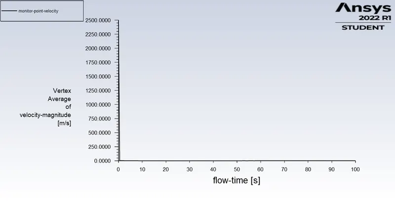
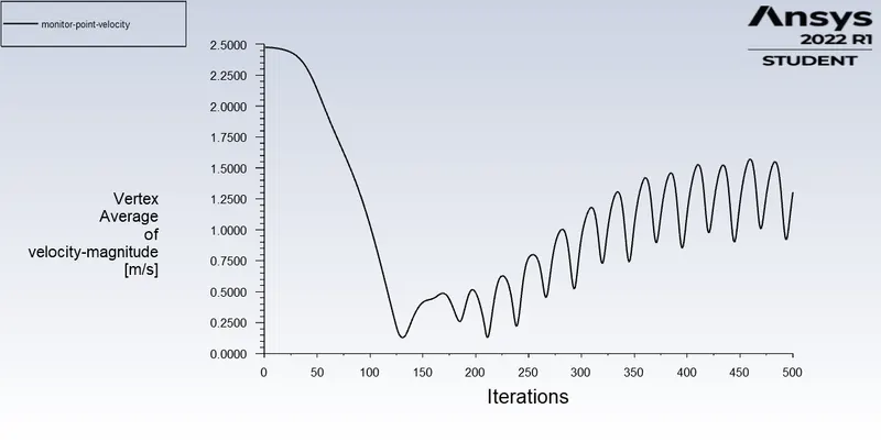
Calculating the strouhal number: velocity at the monitor point report is used to generate the values for the strouhal number plot.

Results:

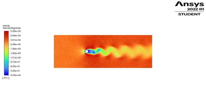
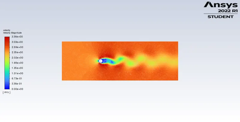
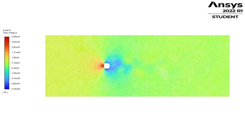
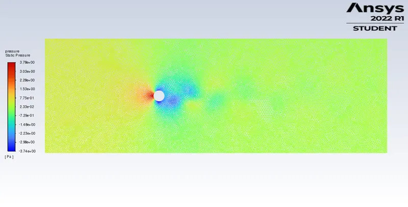
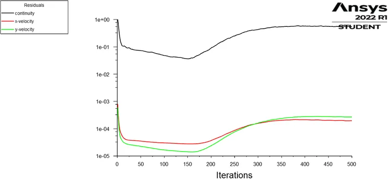
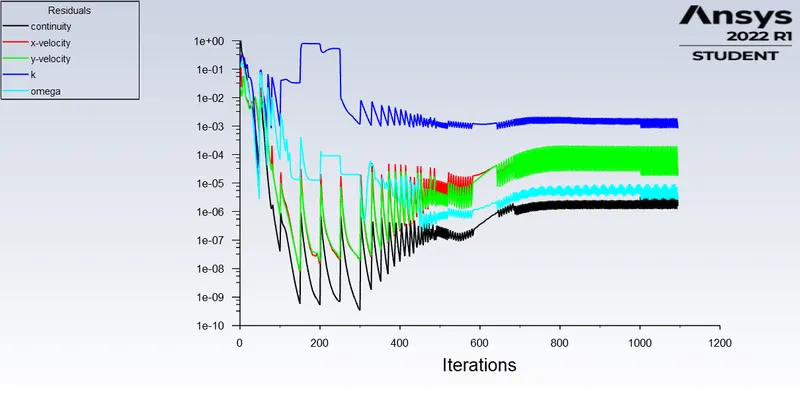
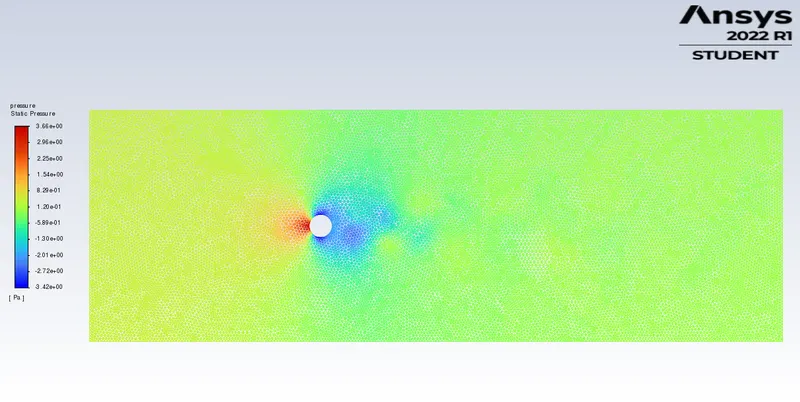
Case-1: Steady vs unsteady case

Reynolds number: 100

Viscosity = 0.05 kg-m/s

Density = 1 kg/m3

Inlet velocity = 2.5 m/s

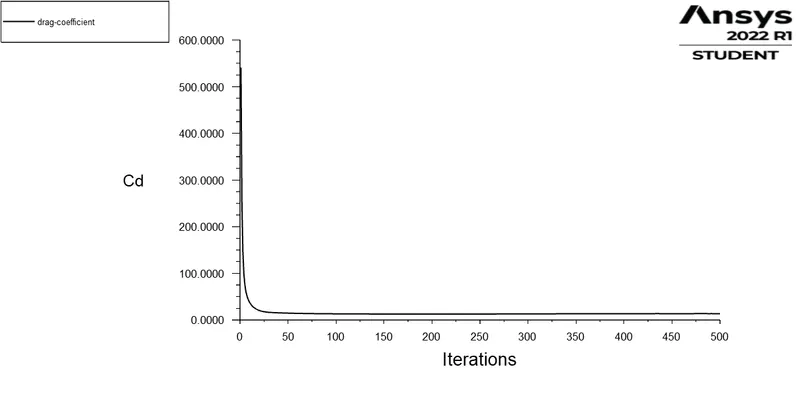
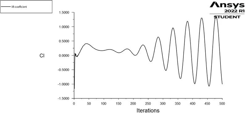
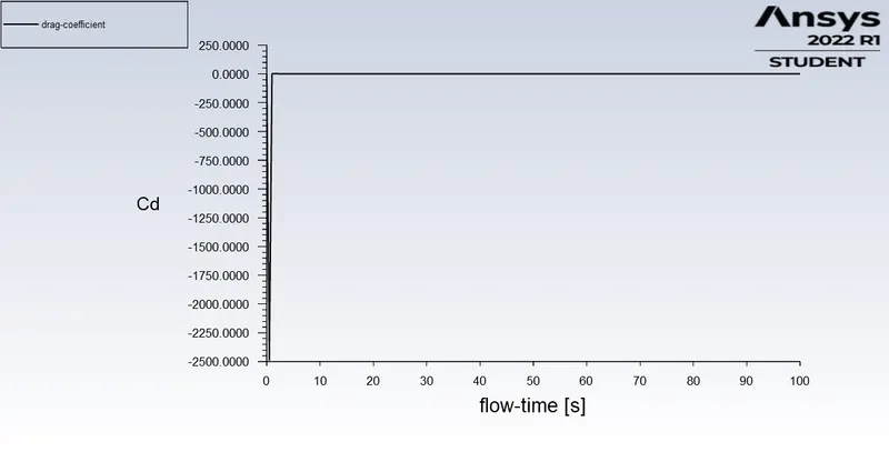
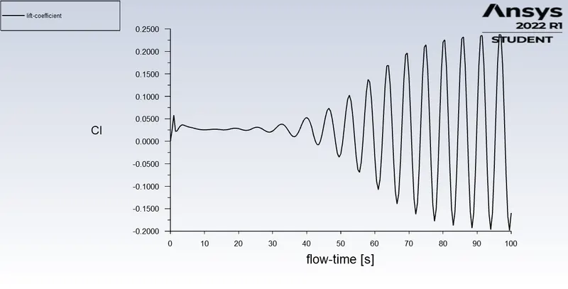
Laminar steady solver Iterations=500	Laminar transient solver Time steps=200 Time step size = 0.5s 50 iterations per time step

Case-2:

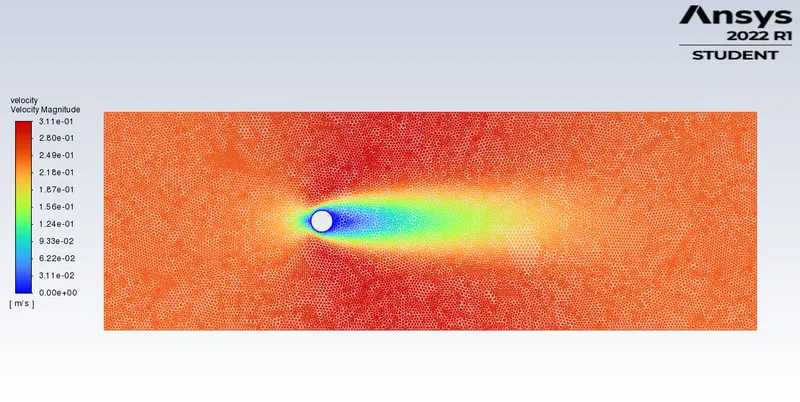
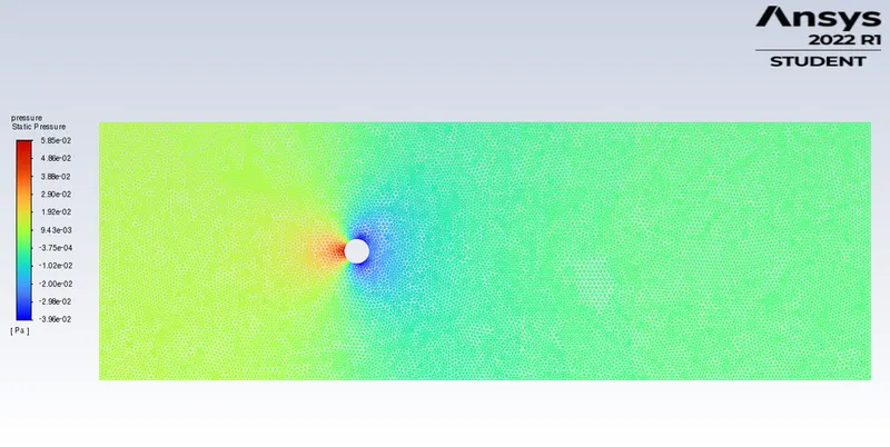
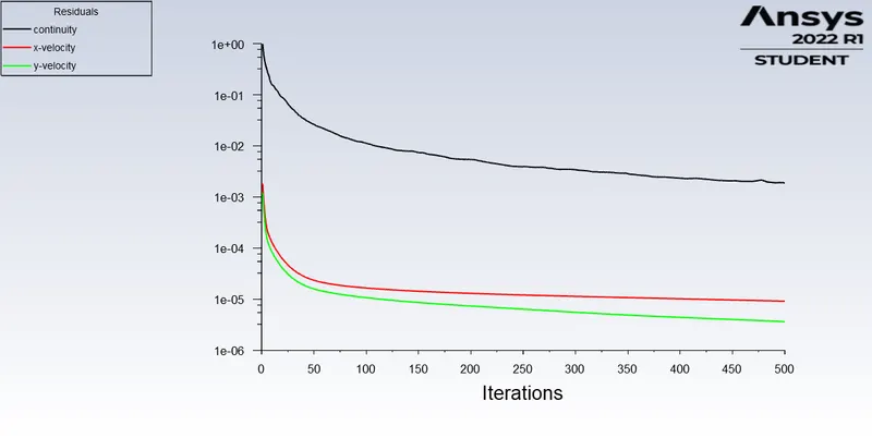
Reynolds number: 10 Viscosity = 0.05 kg-m/s Density = 1 kg/m3	Laminar steady solver Inlet velocity = 0.25 m/s Iterations = 500

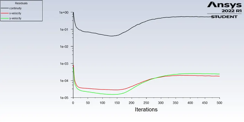
Reynolds number: 100 Viscosity = 0.05 kg-m/s Density = 1 kg/m3	Laminar steady solver Inlet velocity = 2.5 m/s Iterations = 500

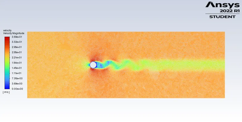
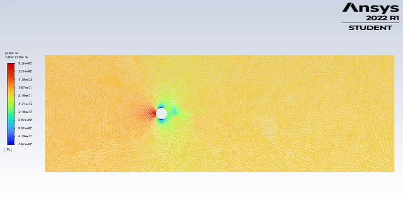
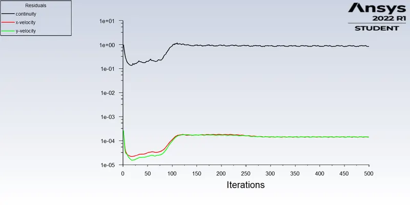
Reynolds number: 1000 Viscosity = 0.05 kg-m/s Density = 1 kg/m3	Laminar steady solver Inlet velocity = 25 m/s Iterations = 500

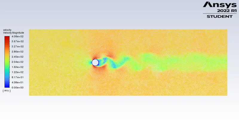
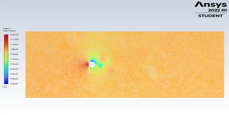
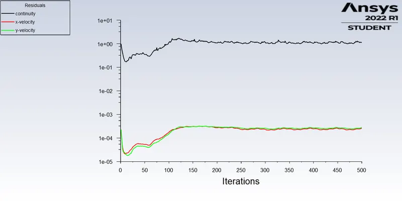
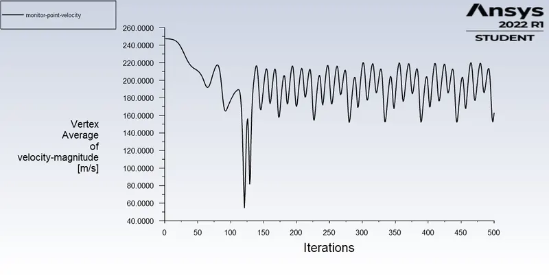
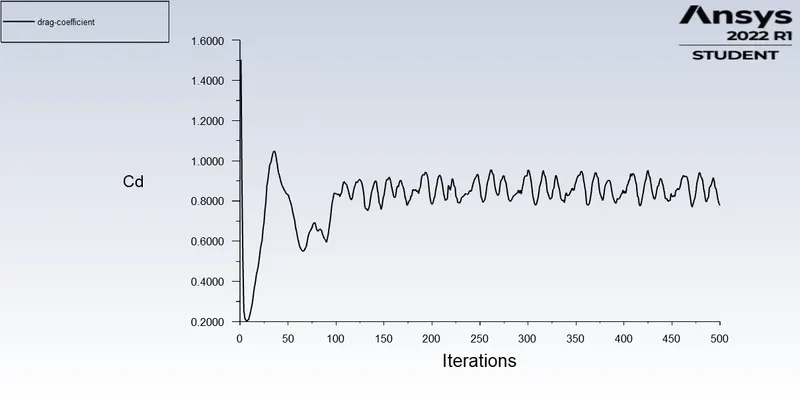
Reynolds number: 10000 Viscosity = 0.05 kg-m/s Density = 1 kg/m3	Laminar steady solver Inlet velocity = 250 m/s Iterations = 500

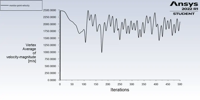
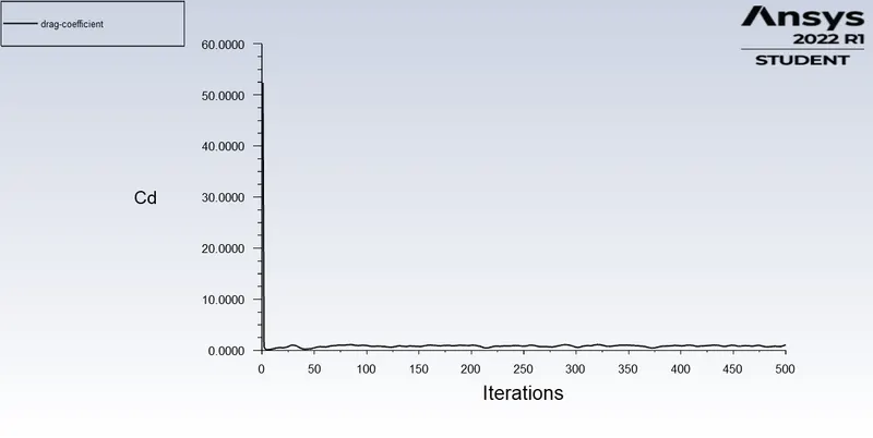
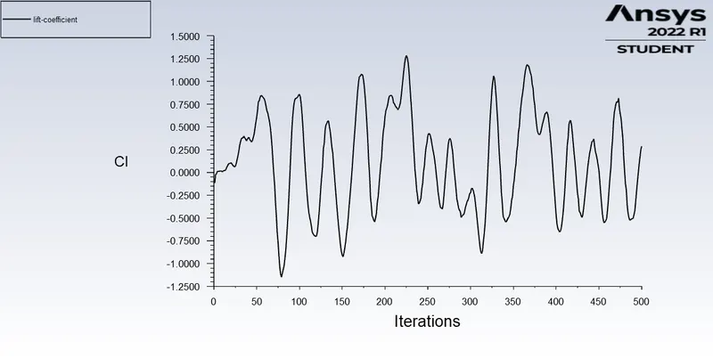
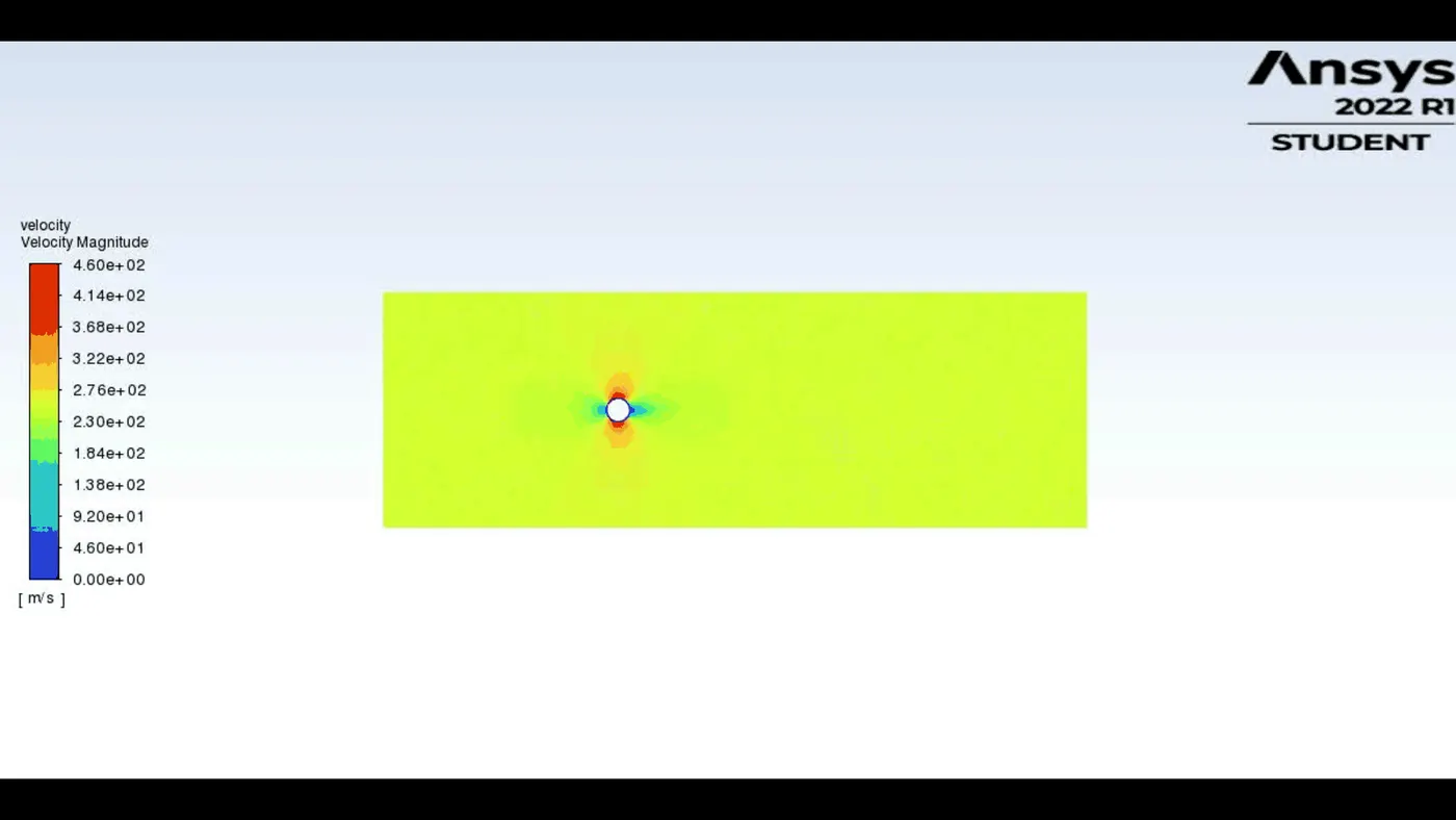
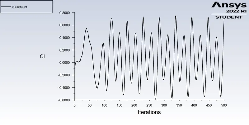
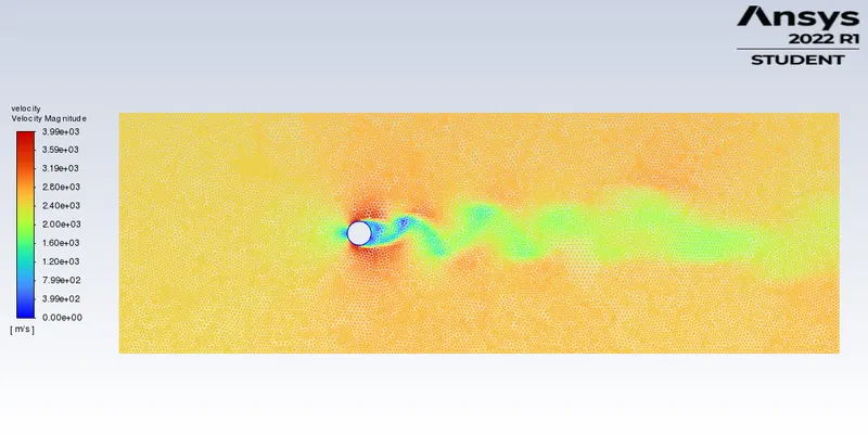
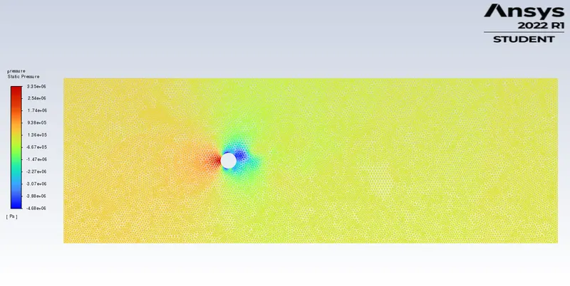
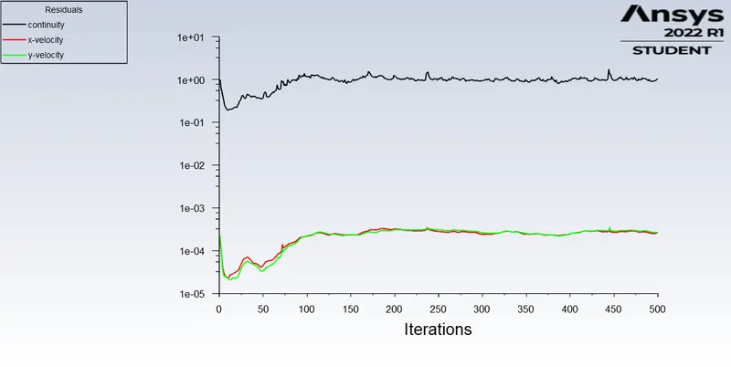
Reynolds number: 100000 Viscosity = 0.05 kg-m/s Density = 1 kg/m3	Laminar steady solver Inlet velocity = 2500 m/s Iterations = 500

Inference:

Case -1:

Steady solver	Cd=1.32	Cl=-0.0056
Transient solver	Cd=1.3627	Cl=-0.159	Strouhal number = 0.38

Case -2:

Reynolds number	Numerical Cd	Numerical Cl
10	3.34	0.0044
100	1.32	-0.0056
1000	0.684	-0.09272
10000	0.778	0.690
100000	1.053	0.2874

Reynolds number	Theoretical Cd	Numerical Cd	Error
Re=10	3.5	3.34	4.57%
Re=100	1.4	1.32	5.71%

Conclusion:

In both the steady and unsteady case, Laminar case, vortex shedding is observed at a reynolds number of 100

In the transient flow, which is time dependant , we are unable to see the flow separation at low reynolds number(below 50), but the phenomenon can be seen once the reynolds number exceeds 100, and the strouhal number is calculated to be 0.38.

When compared with the theoretical Cd value, the error with the numerical value is around 5%.

In the steady case of Re=10, there is no vortex shedding phenomenon.as the flow is laminar with low reynolds number.

In respect with the relation between reynolds number and co-efficient of drag, they have an indirect proportion upto a reynolds number of Re=1000, after that turbulence increases as Re>2000 becomes turbulent and do the Cd values decreases and fluctuates with increase in reynolds number.

Incase of co-efficient of lift, until Re=1000, it keeps on increasing, after that, drops and fluctuates according to the turbulence formation.

Reference:

1. Skrbek, L., & Vinen, W. F. (2009). The Use of Vibrating Structures in the Study of Quantum Turbulence. Progress in Low Temperature Physics, 195–246. doi:10.1016/s0079-6417(08)00004
2. ^{Rajani, B. N., Kandasamy, A., & Majumdar, S. (2009). Numerical simulation of laminar flow past a circular cylinder. Applied Mathematical Modelling, 33(3), 1228–1247. doi:10.1016/j.apm.2008.01.017}