Week 2 - Flow over a Cylinder.

Aim :

To simulate the flow over a cylinder and explain the phenomenon of Karman vortex street.

Objectives :

PART-I

• Simulate the flow with the steady and unsteady case and calculate the Strouhal Number for Re= 100.

PART-II

• Calculate the coefficient of drag and lift over a cylinder by setting the Reynolds number to 10,100,1000,10000 & 100000. (Run with steady solver)
• Discuss the effect of Reynolds number on the coefficient of drag.

Theory :

Phenomenon of Karman vortex street :

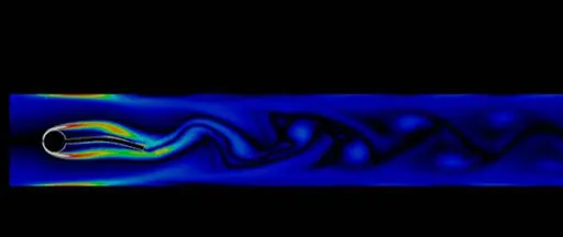
In fluid dynamics, a Kármán vortex street (or a von Kármán vortex street) is a repeating pattern of swirling vortices shedding, caused by a process known as vortex shedding, which is responsible for the unsteady seperation of flow of a fluid around blunt bodies. It is named after the engineer and fluid dynamicist Theodore von Karman.

Physics behind vortex formation :
As a fluid particle flows toward the leading edge of a cylinder, the pressure on the particle rises from the free stream pressure to the stagnation pressure. The high fluid pressure near the leading edge impels flow about the cylinder as boundary layers develop about both sides. The high pressure is not sufficient to force the flow about the back of the cylinder at high Reynolds numbers. Near the widest section of the cylinder, the boundary layers separate from each side of the cylinder surface and form two shear layers that trail aft in the flow and bound the wake. Since the innermost portion of the shear layers, which is in contact with the cylinder, moves much more slowly than the outermost portion of the shear layers, which is in contact with the free flow, the shear layers roll into the near wake, where they fold on each other and coalesce into discrete swirling vortices. A regular pattern of vortices called a vortex street trails aft in the wake.

Drag And Lift :

Figure define the drag and lift direction on an aerofoil shape. It is a common experience that a body meets some resistance when it is forced to move through a fluid. You experience the same feeling when you extend your arm out of the window of a moving car. A fluid may exert forces and moments on a body in and about various directions. The force a flowing fluid exerts on a body in the flow direction is called drag.

A stationary fluid exerts only normal pressure forces on the surface of a body immersed in it. A moving fluid, however, also exerts tangential shear forces on the surface because of the no-slip condition caused by viscous effects. Both of these forces, in general, have components in the direction of flow, and thus the drag force is due to the combined effects of pressure and wall shear forces in the flow direction. The components of the pressure and wall shear forces in the direction normal to the flow tend to move the body in that direction, and their sum is called lift.

The drag and lift forces depend on the density 𝜌 of the fluid, the upstream velocity V, and the size, shape, and orientation of the body, among other things, and it is not practical to list these forces for a variety of situations. Instead, it is more convenient to work with appropriate dimensionless numbers that represent the drag and lift characteristics of the body. These numbers are the drag coefficient CD, and the lift coefficient CL, and they are defined as a formula

The drag and lift forces themselves are not as interesting as the dimensionless drag and lift
coefficients. These depend only on the Reynolds number and an object’s shape, not its
size. The coefficients are defined using the following parameters :
• FD and FL are the drag and lift forces
• rho is the fluid’s density
• Umean is the mean velocity
• A is the projected area (product of thickness and diameter of a cylinder)

SOLVING & MODELLING APPROACH :

Geometry :

2D geometry - showing the flow is passing across a vertical cylender is design in spaceclaim software. Geeneral concideration for fluid control volume is

frontal length - cylender dia(characterstics length ) * 5

Rear length - cylender dia(characterstics length )* 10

Width - cylender dia(characterstics length )*5

this can be achive by using some tools like construction lines, circles, rectangles.

The diamention of fluid domain and cylender is shown below.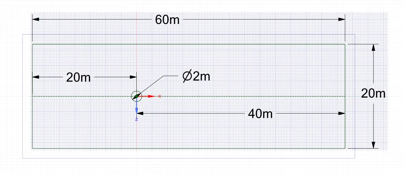

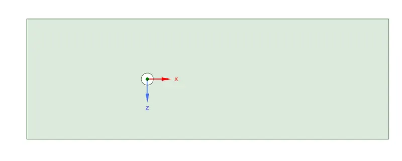
Final geometry is shown below. To design right physics the inside circuler surface is to be deleted to carry out the simulation. Converting the geometry into the surface by using command pull and select.

Meshing :

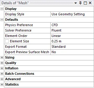
• Now in the mesh mode we set the mesh size, edge sizing and give inflation layers to the cylinder.
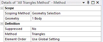
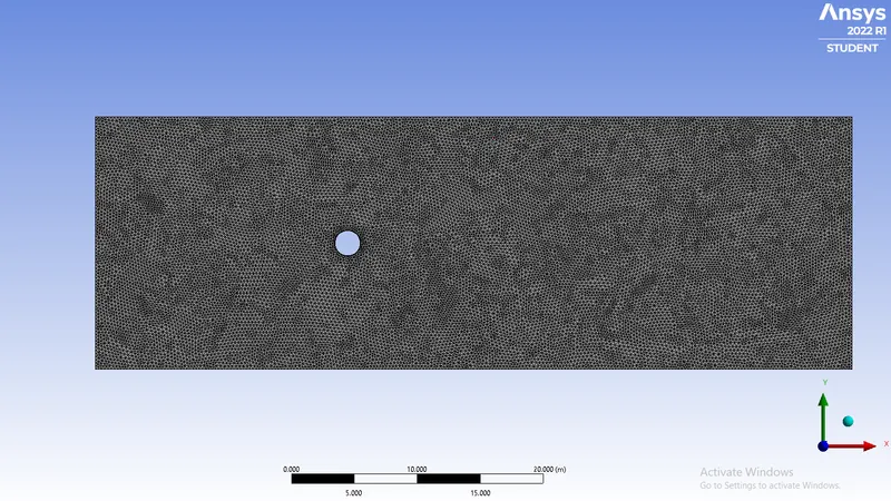
• The mesh size given is 0.25m (Method: Initially, Ansys meshing creates a quadrilateral dominant mesh. We need to convert it into Triangles.

  Go to Mesh→ Insert → Method → Select face → Method(Triangles) →Generate mesh

  
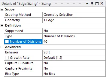
• Edge sizing 4 (Sizing: The cylinder we have is not perfectly circular, so if we proceed like that geometry there might be inaccuracy in results. This option will help us to create smooth curves by dividing the circle into large numbers of edges.

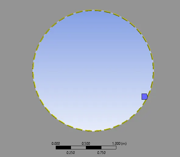
Go to Sizing → Select Edge → Type (Number of divisions) → Enter number and Generate Mesh , after edge sizing image is shown below.

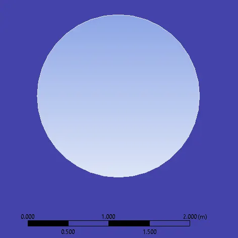
And the obtained mesh is shown below :

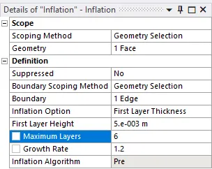
• 6 layers inflation layers with first layer thickness and first layer height of 0.005(Inflation: In order to resolve boundary over the cylinder we will require finner mesh around the cylinder. This option will let us create a finner 'body-fitted mesh' as the flow around the cylinder is quite important.)

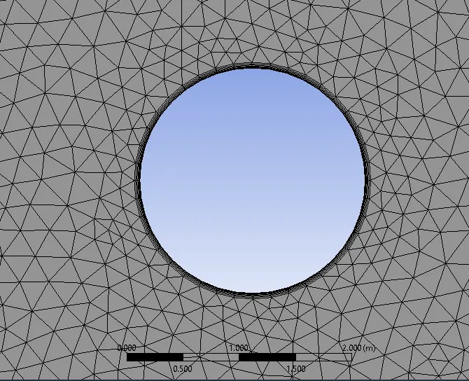
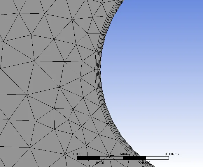
Mesh Quality :

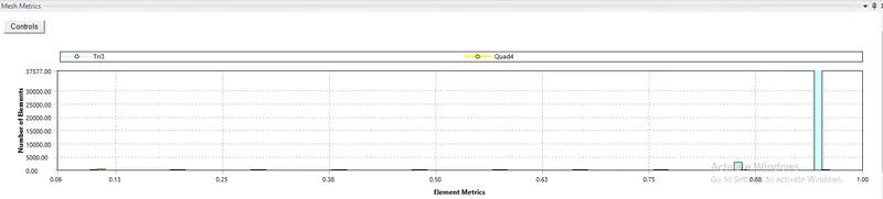
The above graph shows better mesh quality and can obtain mesh independent output which can be used for the simulation.

Name selection :

To set the desired boundaries and to give boundary conditions part naming is to be done after creating the mesh into to the Ansys mesher.

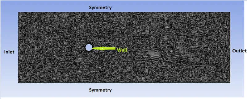
As Shown in above image we can see that as goemetry is symmetric thus symmetry B.C. is used and for cylender no slip wall is used. The naming done according to boundary conditions.

Fluent Setup:

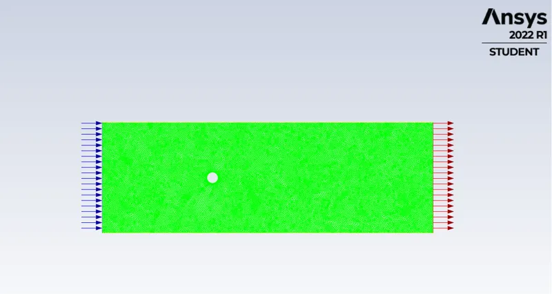
First run Perform Check mesh in order to find any kind of errors in the geometry.

In this simulation we need to perform a vortex shedding formed by flow over a cylender thus we need to set physics according to flow. In vortex sheeding the important parameters are fluid material density and viscocity. This new material is doveloped in the fluent database.

General :

Solver- Pressure Based.
Velocity formulation- Absolute.
Time- Based on the case study we are going to do (Steady/Unsteady).
2D Space- Planer

For time-based simulation we are using the SIMPLE interploation scheme

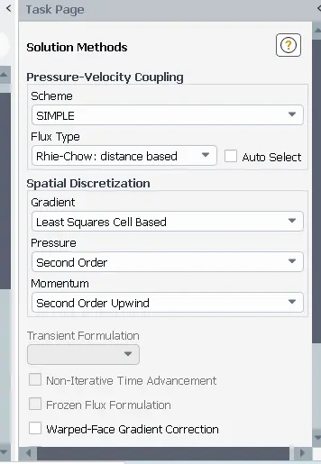
After setting up the whole project hit the calculate and we will get the results that is mentioned in below For the steady state we give the number of iterations and for the unsteady or transient state calculations we give the number of time steps as 500 and the step size is 0.01.

Model :

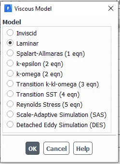
Viscous model- Laminar

Materials :

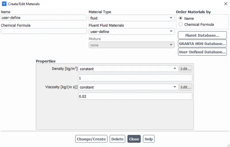
Create/Edit- User_defined_fluid (The fluid is created such that only viscosity will be resopnsible for varing Reynold's number.)

Name- User_defined_fluid
Properties- Density (kg/m3)= 1 (constant)
Viscosity (kg/m-s)= 0.02 (constant)

To check the vortex nature it is important to know the Reynolds no.

Reynolds No :

The Reynolds number is a measure of the ratio of inertial to viscous forces in the flow of a fluid and may be defined as:

Re = ρVD/ μ
where:
ρ = Density,
D = the diameter of the cylinder around which the fluid is flowing,
V = the steady velocity of the flow upstream of the cylinder and
μ = the kinematic viscosity of the fluid.

Using Reynolds no. , viscocity of fluid, density of fluid and cylender dia we can find out the velocity magnitude of flow as mention in above Reynolds No. theory

Boundary Conditions :

Inlet- Velocity Inlet
Velocity Magnitude- for Re = 10--->0.1 m/s

for Re = 100--->1 m/s

for Re = 1000--->10 m/s

for Re = 10000--->100 m/s

for Re = 100000--->1000 m/s

Report Defination :

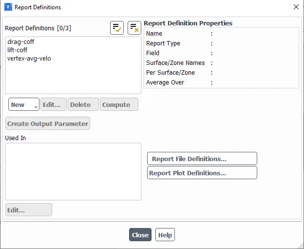
Create a Vertex average of velocity magnitude using surface report at a monitor point 8m away from the center of the cylinder to the right of the cylinder along X-direction.

To read a average velocity value at above monitor point go to definations - surface report - vertex average.

Coefficient of Drag and Coefficient of Lift report created using force report.

For drag go to definations - new - force report - Drag

For lift go to definations - new - force report - Lift

Reference Values :

Plots :

In both i.e. steady and unsteady state simulations, following plots are to be shown:

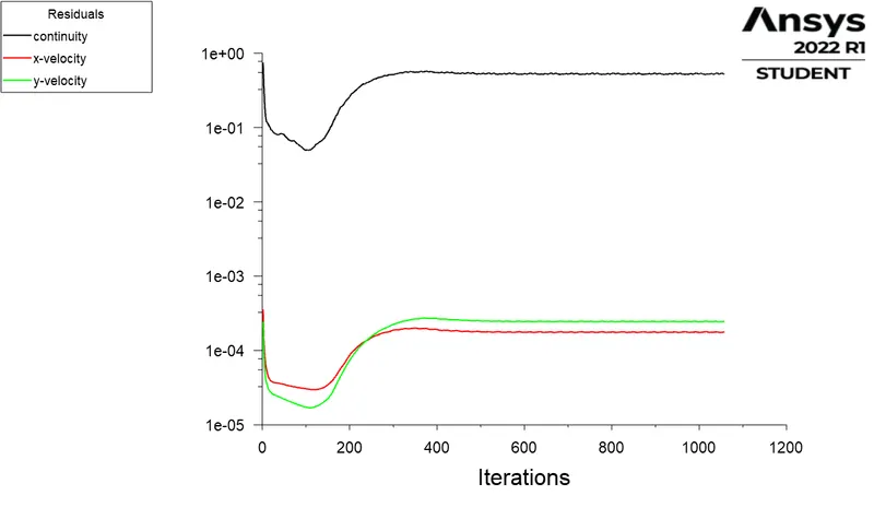
1. Residual plot - This plot helps us in knowing at what point convergence is achieved.

2. Monitor point velocity plot - A monitor point is placed at a distance of 8m from the cylinder in order to calclate the velocity at that point.

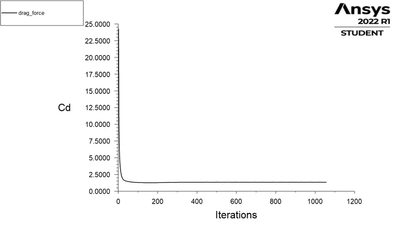
3. Drag coefficient plot - To calculate the drag coefficient.

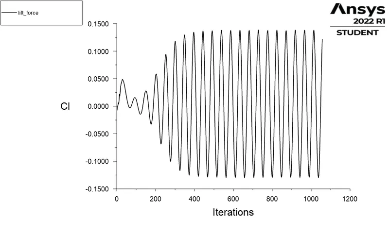
4. Lift coefficient plot - To calculate the lift coefficient.

5. Velocity contour plot - To see the velocity changes in the flow over the cylinder.

6. Contour plots of Pressure & Velocity - Shows the velocity and pressure distribution.

Solution :

Part I : Simulate the flow with the steady and unsteady case and calculate the Strouhal Number for Re= 100.

A. Steady State Flow For Re = 100

Residuals :

Vertex Average of Velocity magnitude :

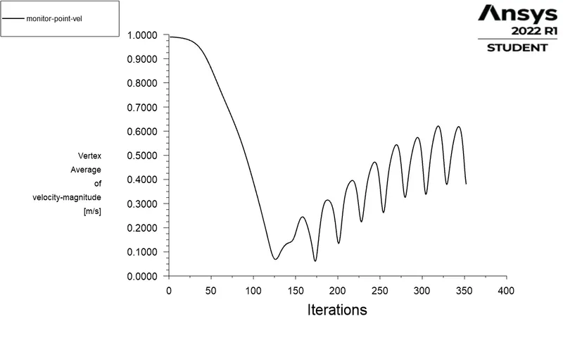
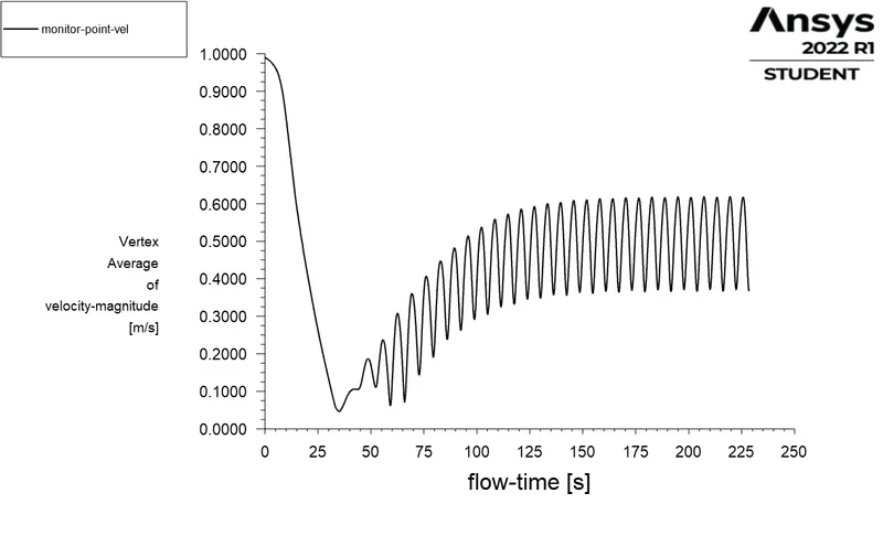
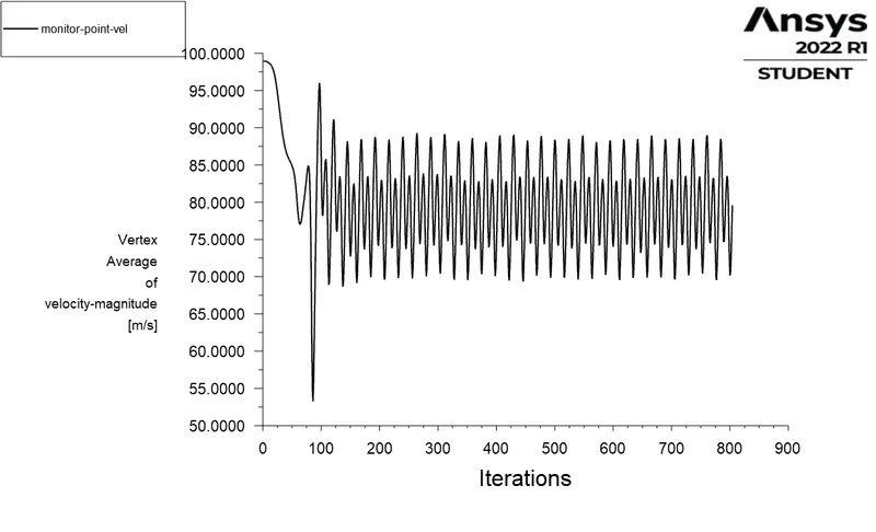
As the flow is showing the vortex sheeding thus the velocity at taken vertex keeps on flucutating with the vortex flow which can be clearly sheen in the graph.

Cofficient of Drag :

Cofficient of Lift :

Velocity Contours :

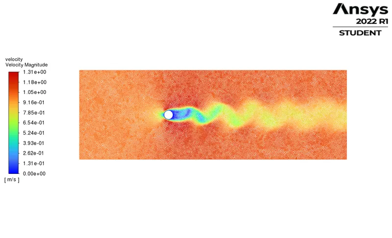
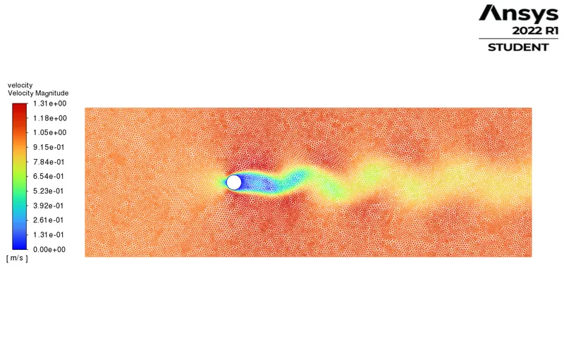
Velocity contours shows that velocity distribution over a flow and there is change in velocity withinin the region which is shown with the help of colour contours. Thus the pattern ov velocity shows vortex shedding behind the cylinder( shown by green region). The vortex sheeding size keeps on increasing with the distence traveled by vortex.

Pressure Contours :

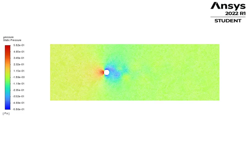
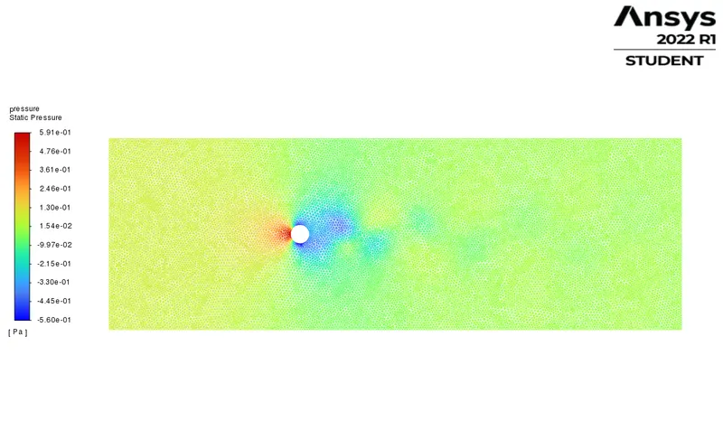
The above contours shows the pressure distribution over a entire domain. Thus when flow impacts the cylender high pressure region is created and as we see aroundthe cylender due to flow seperation the pressure is droped behind and around the cylender.

The above results shows that the flow has reched to steady state as all the residuals are in steady and in a straight lines. The quantity of intrest is Cofficient of drag and cofficient of lift. Drag coff. is also in steady graph but lift coff. shows steadily flucutating graph which is due to wake formation in a flow after cylender. Thus from all of the above results we can say that flow is converged.

Strouhal Number :

The Strouhal Number is a dimensionless value useful for analyzing oscillating unsteady fluid flow dynamics problems.

Strouhal number cannot be calculated for the steady state as there is no time parameter which is required in frequency calculation and can only be calculated for unsteady state condition.

The Strouhal Number can be expressed as

St = w.L/v

where St = Strouhal Number

w = oscillation frequency

L = characteristic frequency

v = flow velocity

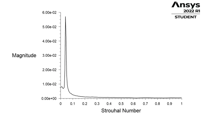
Strouhal number : 4.0100250e-02

Peak magnitude : 5.7073116e-02

B. Unsteady State Flow For Re = 100

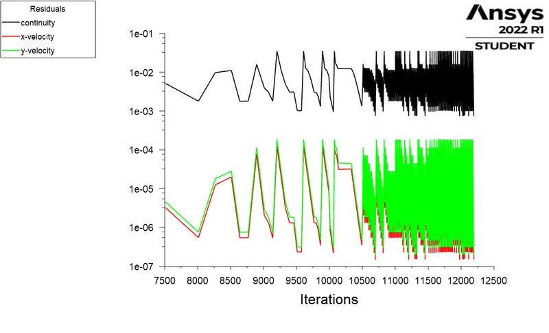
Residuals :

Vertex Average of Velocity magnitude :

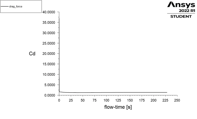
Cofficient of Drag :

Cofficient of Lift :

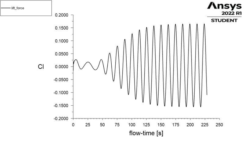
As in unsteady state simulation time is concidered i.e. simulation is recorded since from t= 0 to t= taken time thus the cange for every time step is recorded therefore we can see in the lift cofficent graph that it fluctuation amplitude keeps on increasing till it becomes steady.

Velocity Contours :

Pressure Contours :

Strouhal Number :

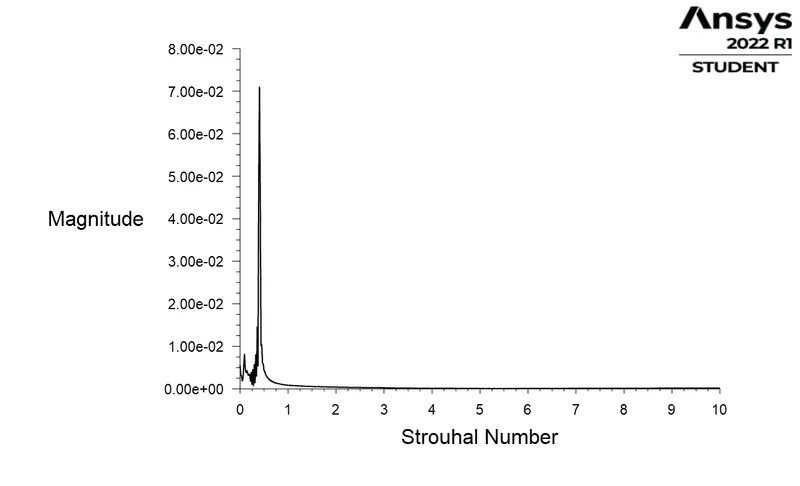
Strouhal number : 4.0593287e-01

Peak magnitude : 7.1038626e-02

Convergence :

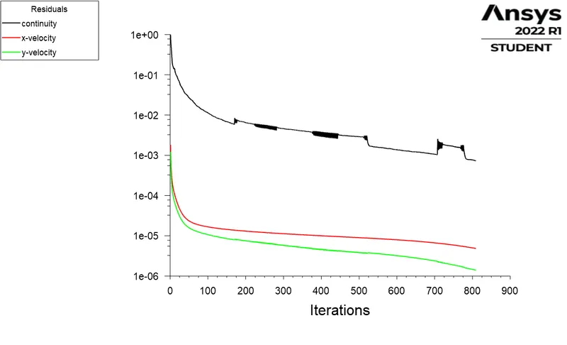
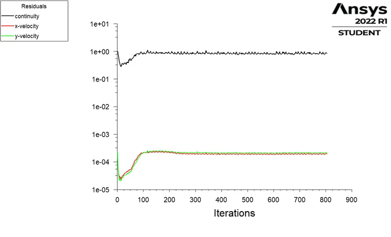
When your simulation has no change on all the convergence criteria, after certain iterations or timesteps, then we can consider that the solution has reached a steady-state, i.e., converged. For CFD, RMS residual levels of 1E-4 are considered to be loosely converged, levels of 1E-5 are considered to be well converged, and levels of 1E-6 are considered to be tightly converged. For complicated problems, however, it's not always possible to achieve residual levels as low as 1E-6 or even 1E-5.

In case Re = 100 Steady state simulation the residuals becomes steady but they didnt fall below 1e-4 thus we go for checking the quantity of intrest which is drag cofficient, lift cofficient and avg. vertex velocity and above graphs shows that all the quantities are in steady state hence we can say solution is converged.

In case Re = 100 unsteady state simulation the residuals are steadily fluctuating but again all of them didnt fall below 1e-4 thus after checking quantity of intrest we can say that solution is converged.

In part two same convergence criteria is choosen and all of the case are converged by looking at the residuals and quantity of interest plots.

Part II

A. Calculate the coefficient of drag and lift over a cylinder by setting the Reynolds number to 10,100,1000,10000 & 100000.

a) Steady state flow for Re = 10

• Residuals :

• Vertex Average of Velocity magnitude :

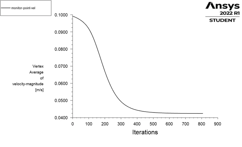
As the flow has very low velocity there is no fluctuations seen in the flow velocity at the designed vertex.

• Cofficient of Drag :

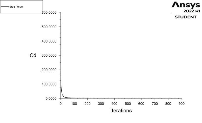
• Cofficient of Lift :

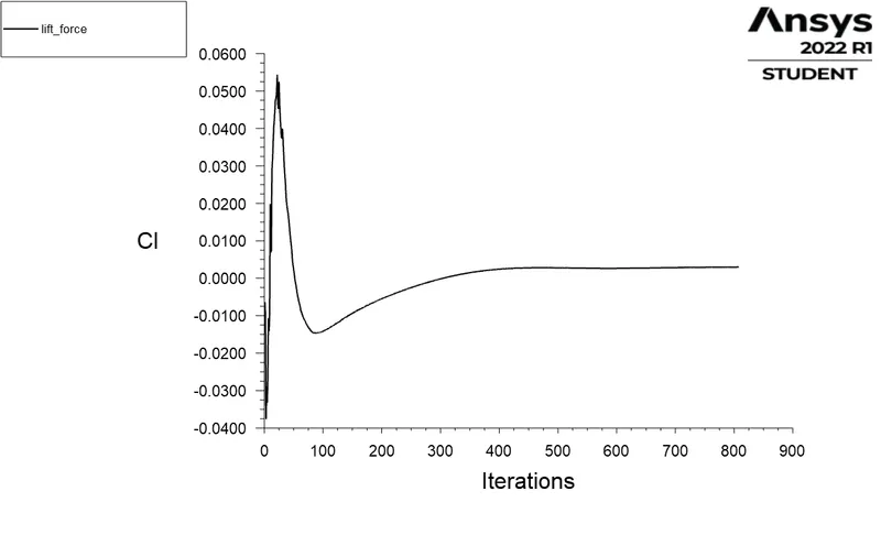
• Velocity Contours :

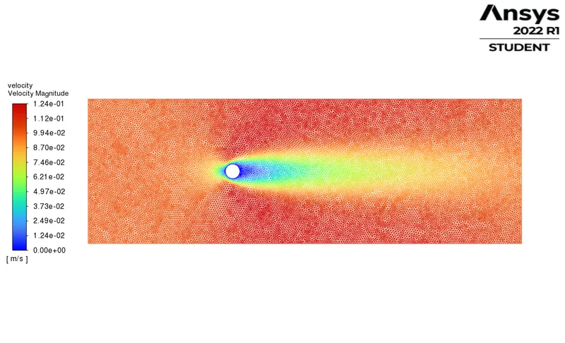
For Re = 10 no vortex shedding effect can be seen in the above velocity contours.

• Pressure Contours :

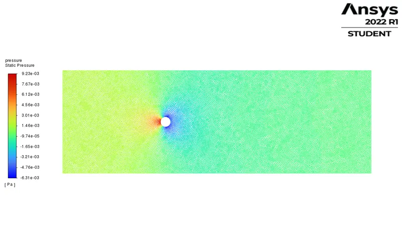
Pressure contours shows the zone of impact which is a high pressure zone within the region and it shows after flow impacting cylender the flow presure reduces.

Due to very low Reynolds no i.e. 10 the vortex shedding effect can not form. To see the vortex shedding, flow should requires higher Reynolds number.

b) Steady state flow for Re = 1000

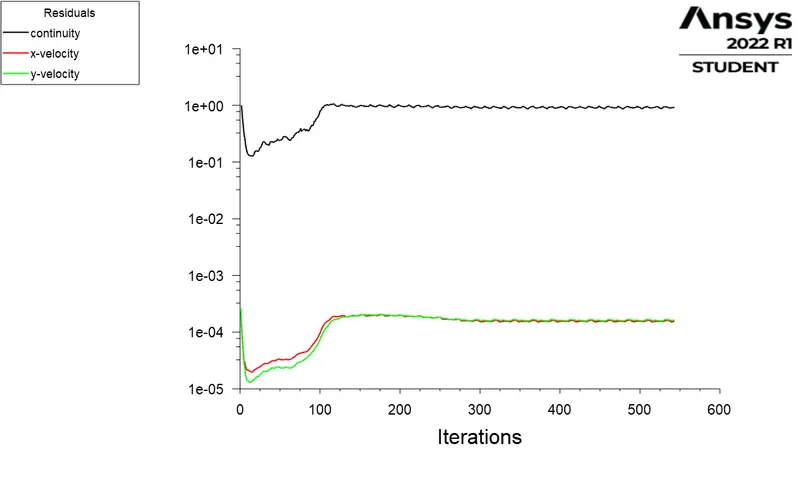
• Residuals :

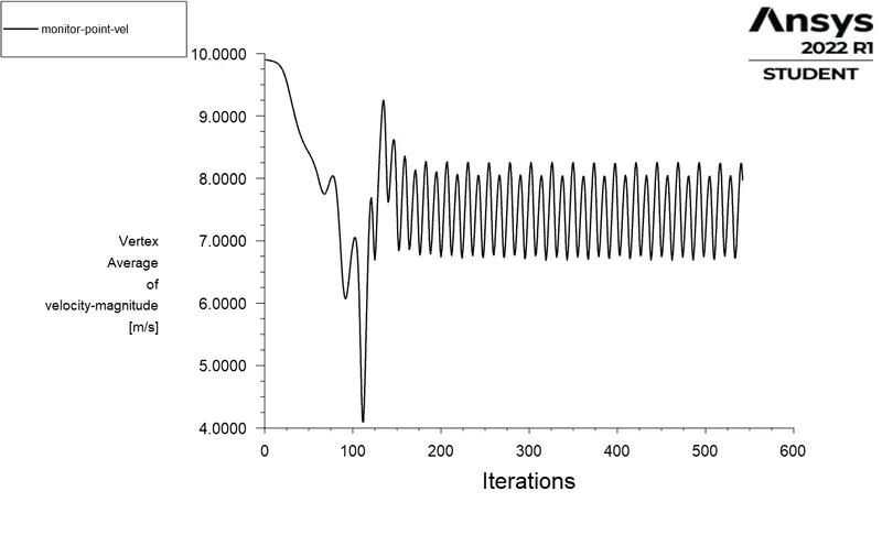
• Vertex Average of Velocity magnitude :

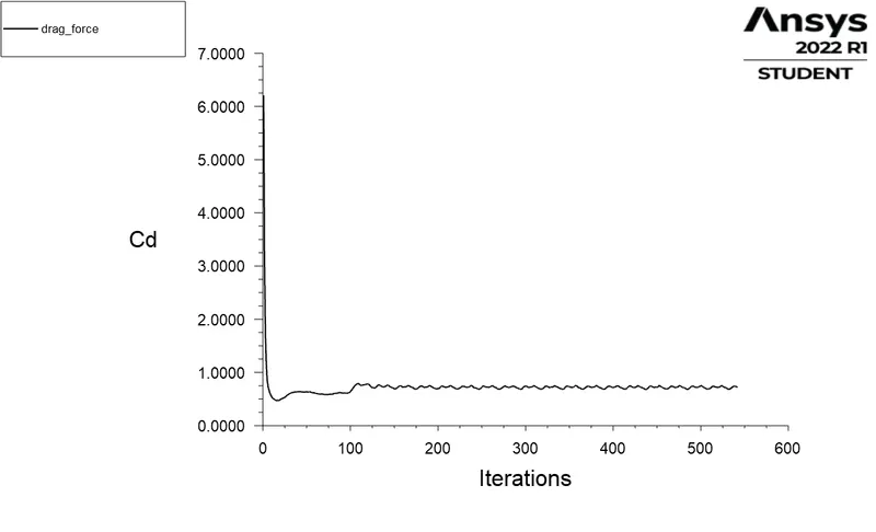
• Cofficient of Drag :

• Cofficient of Lift :

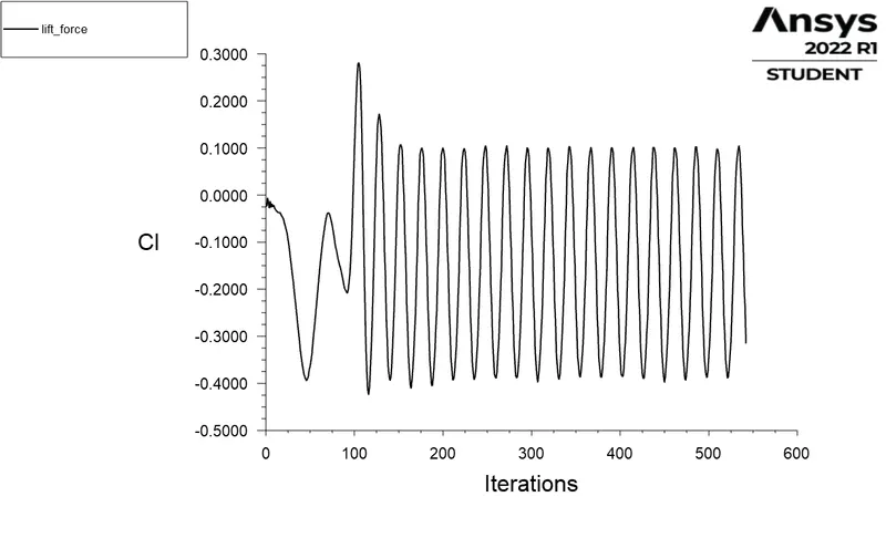
From steady residuals, drag cofficient and the steadily fluctuating avg. vertex velocity and cofficient of lift graph we can say that flow has converged.

• Velocity Contours :

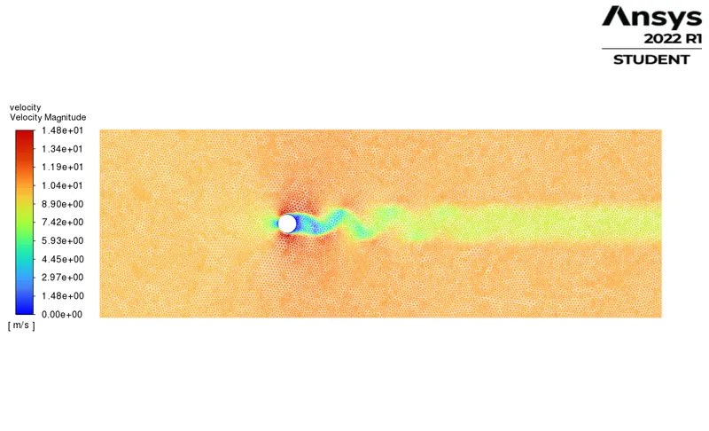
For Re = 1000 we can see in velocity contours that the faster vortex sheeding takes place as the velocity of the flow is increases but the vortex height is reduced as compare to RE = 100.

• Pressure Contours :

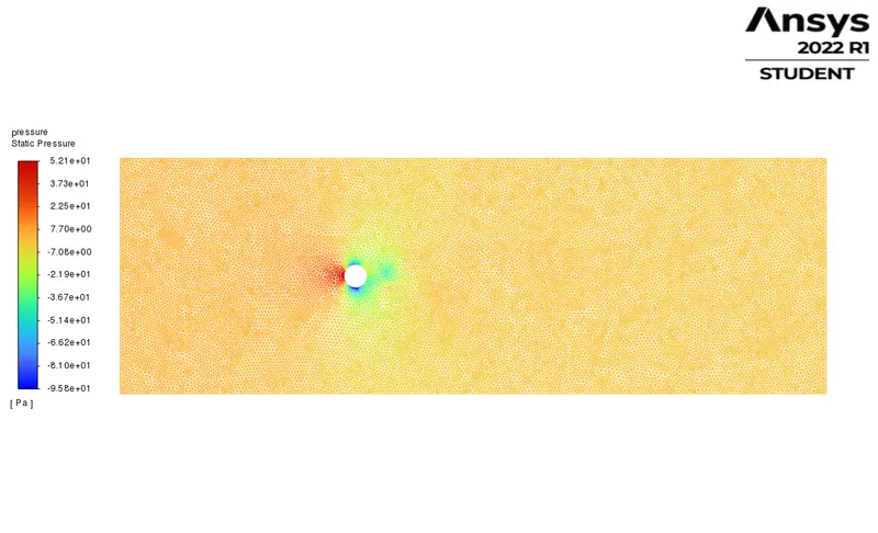
Pressure contours shows that as the flow velocity increases static pressure zone increases with the and flowseperation increases.

c) Steady state flow for Re = 10000

• Residuals :

• Vertex Average of Velocity magnitude :

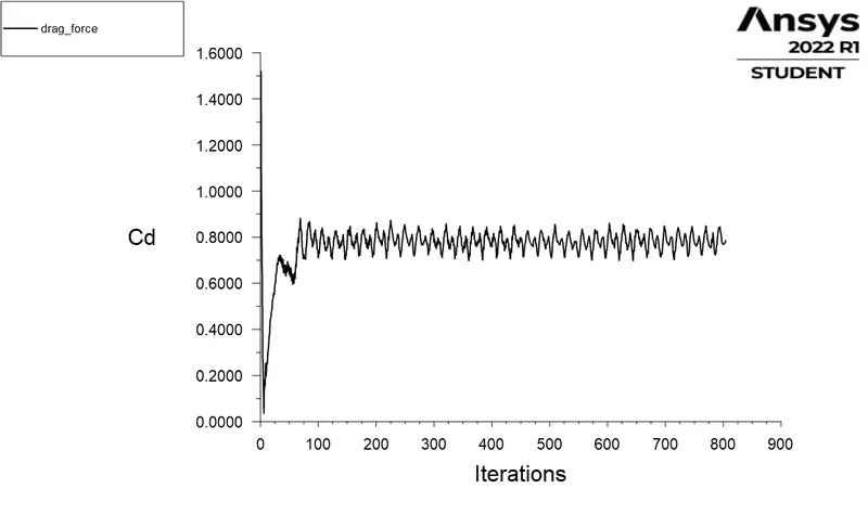
• Cofficient of Drag :

• Cofficient of Lift :

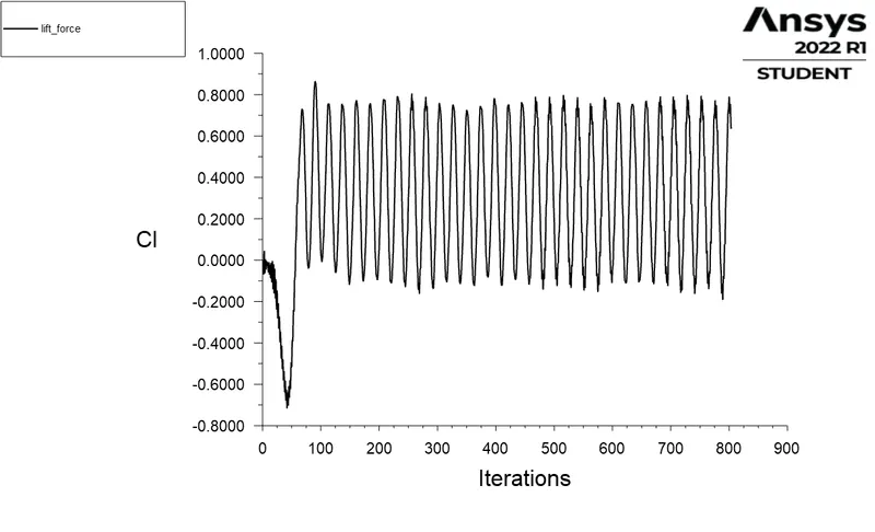
From steady residuals, drag cofficient and the steadily fluctuating avg. vertex velocity and cofficient of lift graph we can say that flow has converged. As the flow reynolds no. increases the the fluctuation in vortex ge faster which can be clearly sheen in vertex avg. velocity and lift cofficient graph.

• Velocity Contours :

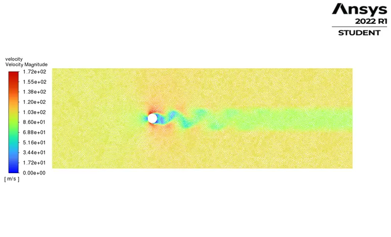
As the reynolds no increases to 10000 the vortex sheeding effect gets more faster but the the effect of vortex or street size keeps on decreasing.

• Pressure Contours :

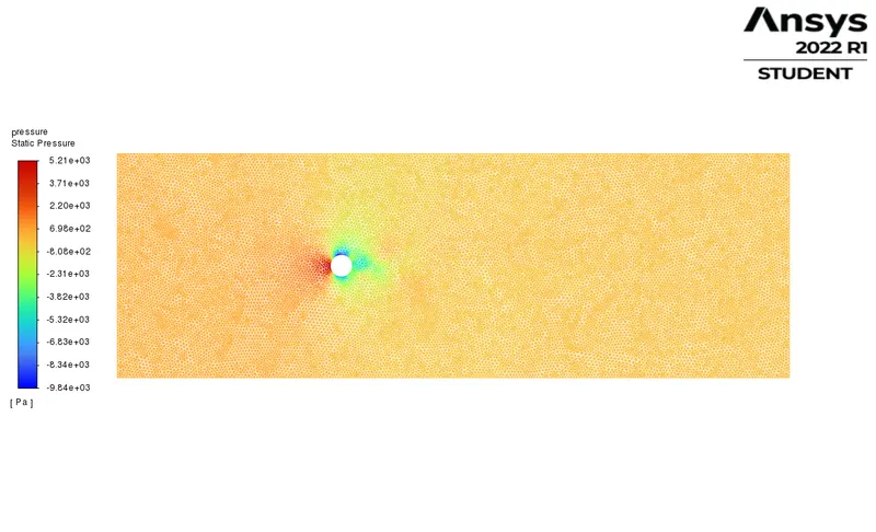
As the reynolds no. increases the pressure of impact decreases and flow seperation increases.

d) Steady state flow for Re = 100000

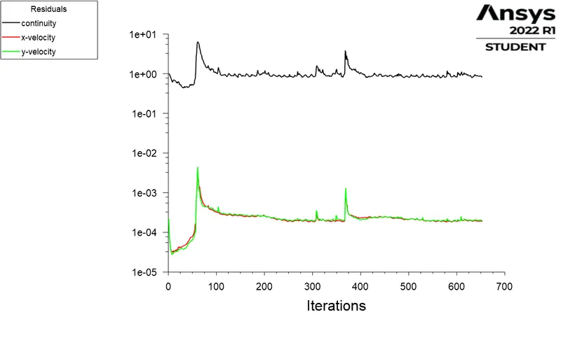
• Residuals :

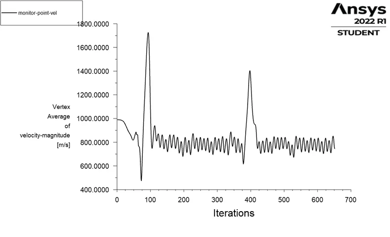
• Vertex Average of Velocity magnitude :

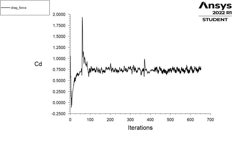
• Cofficient of Drag :

• Cofficient of Lift :

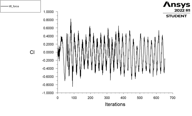
From steady residuals, drag cofficient and the steadily fluctuating avg. vertex velocity and cofficient of lift graph we can say that flow has converged.

• Velocity Contours :

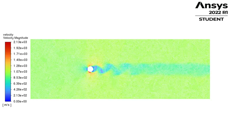
• Pressure Contours :

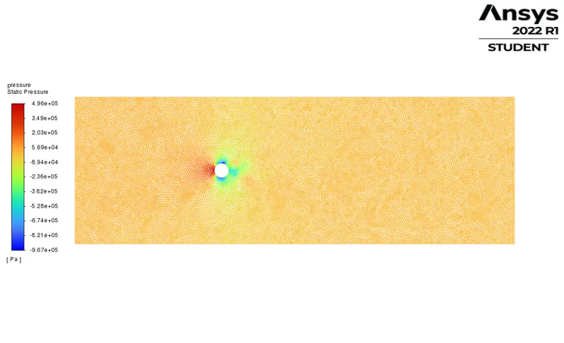
The velocity and pressure contours shows that for RE = 100000 the vortex street formed as compare to case RE = 10000

B. Effect of Reynolds number on the coefficient of drag

Summary Table: Cd and Cl values for the respective reynolds number carried out for the steady state

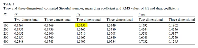
Table From Literature :

Simulation Result Values :

Case	Drag Coefficient	Lift Coefficient	Average velocity at vertex
Re=10	3.3241564	0.00093191	0.042368
Re=100	1.3366762	0.039884041	0.513877
Re=1000	0.73401042	0.24294821	7.589774
Re=10000	0.74729648	0.37316128	81.69005
Re=100000	0.64683046	0.1398	784.5313
Re=100(Unsteady)	1.3203672	0.010078434	0.542187

Comparing above results for RE = with literature [1] - in Literature for Re = 100 cofficient of drag is 1.3353 and from simulation the obtained drag cofficient for RE = 100 is 1.3366762. Thus there is error of 0.1 % in between the literature and simulation value.

Effect of Reynolds Number on Drag Coefficient (Cd) :

Above recorded data is obtained from simulation for variation in reynolds no. . Results shows that as the reynolds no. increases the drag coffficient decreases. Only for case Re = 10000 drag cofficient slightly increase by 0.01.

Trend of variation of Drag Coefficients with Reynold number

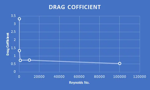
The above graph shows how drag Cofficient is decreases as the Reynolds no. increases.

Conclusion :

• Comparing the steady state and unsteady state solvers for same Reynolds no.- Steady state records the activities as the flow gets stable there is no time factor concideration takes place where as for unsteady state the activities of flow recorded satrting from t = 0. Thus this activities are accordingly captured in given graphs and contours.
• For RE = 10 no vortex shedding street is seen. As we increase the reynolds no. from 100 to 1000 the vortex shedding street is effectively seen. and for Re = 10000 the vortex shedding is very less and street formation is not prominent but for Re = 100000 the vortex street with very small height can be seen.
• As the Reynolds no. increases the cofficient of drag decreases and Lift cofficient increases but for Re = 10000 things get slightly change the drag sightly increases and for Re = 100000 lift is slightly decreases.

References

1. https://www.sciencedirect.com/science/article/pii/S0307904X08000243