Explicit and Implicit Analysis Calculation
OBJECTIVE:
To solve the given equation using implicit and explicit methods with a residual tolerance of 0.01.
Equation: F(u)= u³+9u²+4u
Explicit and Implicit analysis:
1.Explicit Analysis:-
The explicit analysis offers a faster solution in events where there is a dynamic equilibrium or otherwise:
Sum of all forces = mass x acceleration
The explicit method should be used when the strain rates/velocity is over 10 units/second or 10 m/s respectively.
These events can be best exampled by extreme scenarios such as an automotive crash, ballistic event, or even meteor impact. In these cases, the material models do not only need to account for the variation of stress with strain but also the strain rate. On this scale, the strain rates play a particularly important contribution.
Time taken by the explicit analysis depends on wave propagation speed and characteristic length of the element and can predict the time taken for the analysis.
Applications: For wave propagation types of problems such as crash analysis, drop, blast, etc.
2.Implicit Analysis:-
An implicit analysis finds a solution by solving an equation that includes both current and later states of the system
The implicit method should be used when the events are minimal. once the growth of the stress as a function of strain can be Established the solution can be found using implicit analysis.
Sum of all forces = 0
When the problem is nonlinear, the solution is obtained in a number of steps and the solution for the current step is based on the solution from the previous step.
The Implicit Method Takes a lot of time To solve the problem but it is more accurate than the Explicit method.
PROCEDURE:-
Simplification using Explicit Analysis:
The Given Equation F(u) = u³+9u²+4u is calculated by explicit method
Given:
F(u) = u³+9u²+4u
Equation of Stiffness is defined by K=F*u
By Differentiating With respect to the Displacement U we get k(u) We get K(U)= df/du
k(u)=dF/du=3u²+18u+4
The relation ΔF=kΔu can be used to find the incremental displacement.
F- External force.
u- Displacement.
k- Stiffness
ΔF- Incremental force.
Δu- Incremental displacement
Step-1:
F(u)= u³+9u²+4u
K(U)= df/du
k(u)=3u²+18u+4
`K(u_0)`=3(0)²+18(0)+4
`K(u_0)`=4
`Deltau_1`=`DeltaF`/`K(u_0)`
`Deltau_1`=1/4 => 0.25
`Deltau_1`=0.25`
`U_1=Deltau_1+0`
`U_1=0.25`
Sub `U_1=0.25`in Force Function
`F(u_1)=0.25^3+9(0.25)^2+4(0.25)`
`F(u_1) = 1.578`
`F_(external)`=`Delta F`= 1
`F_(Internal)`l=1.578
```Residual (R^0)=(F_(Internal))_1-(F_(external))_1=1.5781-1``
`Residual (R^0)=0.578`
`U_(exact)=0.177`
Step-2:
F(u)= u³+9u²+4u
K(U)= df/du
k(u)=3u²+18u+4
`K_(u1)=3(0.25)²+18(0.25)+4`
`K_(u1)=8.6875`
`Deltau_2`=`DeltaF`/`K(u_1)`
`Deltau_2`=1/8.6875`
`Deltau_2`=0.115`
`U_2=Deltau_2+ U_1`
`U_2=0.115+0.25`
`U_2=0.365`
Sub `U_2=0.365`in Force Function
`F(u_2)=0.365^3+9(0.365)^2+4(0.365)`
`F(u_2) = 2.707`
`F_(external)`=`Delta F`= 1+1`
`F_(Internal)`2= 2.707`
```Residual (R^0)=(F_(Internal))_2-(F_(external))_2=2.707-2`
`Residual (R^0)=0.707`
`U_(exact)=0.296`
Step-3:
F(u)= u³+9u²+4u
K(U)= df/du
k(u)=3u²+18u+4
`K_(u2)=3(0.365)²+18(0.365)+4`
`K_(u_2)=10.969`
`Deltau_3`=`DeltaF`/`K(u_2)`
`Deltau_3`=1/10.969`
`Deltau_3`=0.0911`
`U_3=Deltau_3+ U_2`
`U_3=0.0911+0.365`
`U_3=0.456`
Sub `U_3=0.456`in Force Function
`F(u_3)=0.456^3+9(0.456)^2+4(0.456)`
`F(u_3) = 3.792`
`F_(external)`=`Delta F`= 1+1+1`
`F_(Internal)`3= 3.792`
```Residual (R^0)=(F_(Internal))_3-(F_(external))_3=3.792-3`
`Residual (R^0)=0.792`
`U_(exact)=0.391`
The `U_(exact)` values are obtained by Solving External energy values in the Quadratic Equation. `ax^3+bx^2+cx+d`
a=1; b=9; c=4; d=`DeltaF`
Table-1: Summary of explicit Analysis:
| Step-1 | `Deltaf_i` | `Deltau_i` | `U_i` | `(F_(ext))_i` | `(F_(Int))_i` | `(R^0)=(F_(ext))_i-(F_(Int))_i`` | `U_(exact)` |
| 1 | 1 |
0.25 |
0.25 | 1 | 1.578 | 0.578 | 0.177 |
| 2 | 1 | 0.115 | 0.365 | 2 | 2.707 | 0.707 | 0.296 |
| 3 | 1 | 0.091 | 0.446 | 3 | 3.792 | 0.792 | 0.391 |
From The table, we can see that internal energy and external energy are not in an equilibrium state. As the internal energy per step is not equal to the applied external energy.
IMPLICIT ANALYSIS:
An implicit analysis is the same as an explicit analysis, except that at the end of each stepNewton-Raphson iterations are used to enforce equilibrium before moving to the next step.
Basically, an incremental force is applied to advance the solution forward at the beginning of a step. However, internal forces and external forces will not be in equilibrium unless the stiffness is linear for the given step.
Hence, in order to achieve equilibrium, corrections must be made to the displacement. This is accomplished by using Newton-Raphson iterations to minimize the residual, `R(u)=f_(Int)-F_(ext)`
By neglecting higher-order terms in the series, setting Rj+1 = 0, and solving for δuj+1 the following correction is obtained.
`deltau^(j+1) =-[K(u^j)]^-1*R^j`
Iteration variable is j and it may take several iterations for the norm of the residual, `||R||`, to be reduced below the chosen tolerance criteria (for the example below a tolerance of `10^-2`is chosen).
Step-1:
F(u)= u³+9u²+4u
K(U)= df/du
k(u)=3u²+18u+4
`K(u_0)`=3(0)²+18(0)+4
`K(u_0)`=4
`Deltau_1`=`DeltaF`/`K(u_0)`
`Deltau_1`=1/4 => 0.25
`Deltau_1`=0.25`
`U_1=Deltau_1+0`
`U_1=0.25`
Sub `U_1=0.25`in Force Function
`F(u_1)=0.25^3+9(0.25)^2+4(0.25)`
`F(u_1) = 1.578`
`F_(external)`=`Delta F`= 1
`F_(Internal)`l=1.578
```Residual (R^0)=(F_(Internal))_1-(F_(external))_1=1.5781-1``
`Residual (R^0)=0.578`
Here `Residual (R^0)=0.578` is greater than `10^-2` so the Newton-Raphson iterations are applied to the function.
Let us consider `U_1=U_1^0`
`deltau^1=-[k(u_1^0)]^-1*R^0`
`(u_1^0)=3u^2+18u+4`
Sub `u_1^0=0.25`
`k(u_1^0)=3(0.25)^2+18(0.25)+4`
`k(u_1^0)=8.6875`
`deltau^1= -0.578/8.6875`
`deltau^1= -0.066`
`u_1^(1)=deltau^1+u_1^0`
`u_1^1=-0.066+0.25`
`U_1^1=0.184`
Sub `U_1^1=0.184` in the function F(u)=`u^3+9u^2+4u`
`F(u_1^1)= (0.184)^3+9(0.184)^2+4(0.184)`
`F(u_1^1)=1.046`
`R^1= F_(Internal)-F_(external)`
`R^1=1-0.046`
`R^1=0.046`
( which is still less than `10^-2`) Another iteration is Applied.
Iteration-2
Let us consider `U_1=U_1^1`
`deltau^2=deltau^1-[k(u_1^1)]^-1*R^1`
`u_1^1=0.184`
Sub `K(u_1^1)=0.184` in K(u) function
`K(u_1^1)=3(0.184)^2+18(0.184)+4`
`K(u_1^1)=7.413`
`deltau^2=deltau^1-[k(u_1^1)]^-1*R^1`
`deltau^2=-0.066-[7.413]^-1*0.046`
`deltau^2=-0.072`
`U_1^2=deltau^2+U_1^0`
`U_1^2=0.178`
`F(U)=u^3+9u^2+4u`
`F(U)=(0.178)^3+9(0.178)^2+4(0.178)`
`F(U)=1.002`
`R^2= F_(Int)-F_(ext)`
`R^2= 1.002-1`
`R^2= 0.002`
Since `R^2=0.002` is less than `10^-2` The iteration can be stopped here.
`U_(exact)=0.177`
Step-2:
F(u)= u³+9u²+4u
K(U)= df/du
k(u)=3u²+18u+4
Sub `K(u_1)=0.178` in equation.
`K(u_1)`=3(0.178)²+18(0.178)+4`
`K(u_1)`=7.29`
`Deltau_2`=`DeltaF`/`K(u_1)`
`Deltau_2`=1/7.29`
`Deltau_2=0.137`
`U_2=Deltau_2+U_1^2`
`U_2=0.137+0.178`
`U_2=0.315`
Sub `U_2=0.315`in Force Function
`F(u_2)=(0.315)^3+9(0.315)^2+4(0.315)`
`F(u_2) = 2.184`
`F_(external)`=`Delta F`= 1+1`
`F_(Internal)`l=2.184`
```Residual (R^0)=(F_(Internal))_1-(F_(external))_1=2.184-2`
`Residual (R^0)=0.184`
Here `Residual (R^0)=0.184` Is greater than `10^-2` so the Newton-Raphson iterations are applied to the function.
Let us consider `U_1=U_1^0`
`deltau^1=-[k(u_2^0)]^-1*R^0`
`K(u_2^0)=3u^2+18u+4`
Sub `K(u_2^0)=0.315`
`k(u_2^0)=3(0.315)^2+18(0.315)+4`
`k(u_2^0)=9.967`
`deltau^2= -0.184/9.967`
`deltau^2= -0.018`
`u_2^(1)=deltau^2+u_2^0`
`u_2^1=-0.018+0.315`
`U_2^1=0.297`
Sub `U_2^1=0.297` in the function F(u)=`u^3+9u^2+4u`
`F(u_2^1)= (0.297)^3+9(0.297)^2+4(0.297)`
`F(u_2^1)=2.007`
`R^1= F_(Internal)-F_(external)`
`R^1=2-2.007`
`R^1=0.007`
Since `R^1=0.007` is less than `10^-2` No further iterations are needed as it achieved the Convergence.
`U_(exact)=0.296`
Step-3:-
F(u)= u³+9u²+4u
K(U)= df/du
k(u)=3u²+18u+4
Sub `K(u_2)=0.297` in equation`
`K(u_2)`=3(0.297)²+18(0.297)+4`
`K(u_2)`=9.61`
`Deltau_3`=`DeltaF`/`K(u_2)`
`Deltau_3`=1/9.61`
`Deltau_3=0.104`
`U_3=Deltau_3+U_2`
`U_3=0.104+0.297`
`U_3=0.401`
Sub `U_3=0.401`in Force Function
`F(u_3)=(0.401)^3+9(0.401)^2+4(0.401)`
`F(u_3) = 3.115`
`F_(external)`=`Delta F`= 1+1+1`
`F_(Internal)=3.115`
```Residual (R^0)=(F_(Internal))_1-(F_(external))_1=3.115-3`
`Residual (R^0)=0.115`
Here `Residual (R^0)=0.115` Is greater than `10^-2` so the Newton-Raphson iterations are applied to the function`
Let us consider `U_2=U_2^0`
`deltau^3=-[k(u_3^0)]^-1*R^0`
`K(u_3^0)=3u^2+18u+4`
Sub `K(u_3^0)=0.401`
`k(u_3^0)=3(0.401)^2+18(0.401)+4`
`k(u_3^0)=11.7`
`deltau^3= -0.115/11.7`
`deltau^3= -0.009`
`u_3^(0)=deltau^3+u_3^0`
`u_3^0=-0.009+0.401`
`U_3^0=0.391`
Sub `U_3^0=0.391` in the function F(u)=`u^3+9u^2+4u`
`F(u_3^0)= (0.391)^3+9(0.391)^2+4(0.391)`
`F(u_3^0)=2.993`
`R^1= F_(Internal)-F_(external)`
`R^1=3-2.993`
`R^1=0.002`
`since `R^1=0.002` is less than `10^-2` No further iterations are needed as it achieved the Convergence.
`U_(exact)=0.391`
The `U_(exact)` values are obtained by Solving External energy values in the Quadratic Equation. `ax^3+bx^2+cx+d`
a=1; b=9; c=4; d=`DeltaF`
Table-2: Summary of Implicit Analysis:
| Step-1 | `Deltaf_i` | `Deltau_i` | `(F_(ext))_i` | `(F_(Int))_i` | `(R^0)=(F_(ext))_i-(F_(Int))_i`` | `U_(exact)` |
| 1 | 1 |
0.178 |
1 | 1.002 | 0.002 | 0.177 |
| 2 | 1 | 0.297 | 2 | 2.007 | 0.007 | 0.296 |
| 3 | 1 | 0.391 | 3 | 2.993 | 0.002 | 0.391 |
From the table, we can see that the external and internal forces are Converged before skipping to the next cycle from one cycle.
Although the Internal and external energy Are not in equilibrium in Both Methos, Implicit has fewer errors compared with explicit this is because The analysis moves to the next step only when the convergence is achieved in the first step, thus the errors are small.
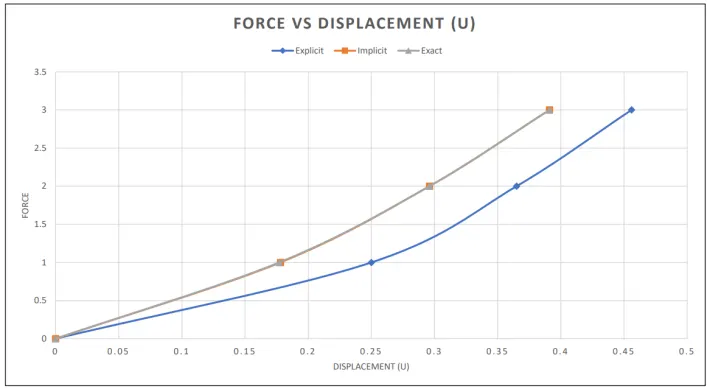
The results of explicit and Implicit are summarized in the table below.
| Step-`i` | Force | Explicit | Implicit | Exact |
| 0 | 0 | 0 | 0 | 0 |
| 1 | 1 | 0.25 | 0.178 | 0.177 |
| 2 | 2 | 0.365 | 0.297 | 0.296 |
| 3 | 3 | 0.456 | 0.391 |
0.391 |
Graph:-
Results:-
Thus from the graph, the Implicit values and the exact values go the same, and the explicit analysis drifts from the exact solution. The reason for the change in drift is because of the lack of equilibrium between Internal and external energies. As in the Implicit analysis, the Newton Raphson Iterations are used for Convergence So that they can Replicate the exact solution According to the Given tolerance and the solution is achieved by the Iterations. that is clearly shown in the Graph as the Implicit and Exact solutions lies exactly on the same track.