Week - 2 - Explicit and Implicit Analysis

Aim: The objective of this assignment is to demonstrate the use of explicit and implicit numerical methods in solving the given function.

Explanation: The numerical method of solving a non-linear equation involves solving it in a sequence of time steps.

In the explicit method, used for dynamic scenarios, the value of the function at an incremental step is derived from the value at the previous time step. In an explicit scheme. The matrix equation being solved is in the following form.

[M][x'']+[C][x']+[K][x]=[c]

Here, the constant matrices are diagonal matrices that can be easily inverted.

The implicit method is used in static/quasi-static scenarios, where internal and external forces are supposed to be in equillibrium. In order to achieve convergence of the solution, an incremental force in the form of a Newton-Raphson iteration is applied. The value of the function at a time step requires information from both the current and the previous time step. The matrix equation being solved is in the following form.

[K][x]=[c]

Since there are no acceleration or velocity components, the implicit method is not suitable for dynamic scenarios. Here, the stiffness matrix is not a diagonal matrix. Thus, it cannot be easily inverted, as a result of which, the implicit method requires more computations and takes longer.

Calculation: The function being solved for is F(u)=u^3+9u^2+4u with a tolerance of 10^-2.

The stiffness that can be derived from this function is k(u) = dF(u)/du = 3u^2+18u+4

The results and graphs are shown both here and in an excel spreadsheet enclosed with this assignment.

1) Explicit method: The explicit method here makes use of incremented external force steps (del F). The procedure of deriving displacement (u)and resultant internal force (f(u)) is listed below.

• Initial value of displacement (u0) is considered to be 0, i.e. u0=0.
• Stiffness at u0 is given by k(u0) = (3*0)+(18*0)+4 = 4
• The first increment in displacement is given by del u1 = del f/k(u0) = 1/4 = 0.25
• The next step in displacement is given by u1 = u0+del u1 = 0+0.25 = 0.25
• The internal force at this displacement is given by f(u1) = (0.25^3)+9(0.25^2)+(4*0.25) = 1.578
• The next displacement step (u1) is considered for the next set of calculations.
• The stiffness, increment in displacement, next displacement step and internal force is re-evaluated at this new displacement step.
• All the above steps are repeated until data at 5 displacements are derived.

2) Implicit method: The implicit method uses the same set of steps as the explicit method with the addition of a residual correction factor (Newton-Raphson iteration) for ensuring force equillibrium. The procedure for deriving the displacement and resultant internal forces is listed below.

• Initial value of displacement (u0) is set as u0 = 0
• Stiffness at u0 is given by k(u0) = (3*0)+(18*0)+4 = 4
• The first increment in displacement is given by del u1 = del f/k(u0) = 1/4 = 0.25
• The next step in displacement is given by u1 = u0+del u1 = 0+0.25 = 0.25
• The internal force at this displacement is given by f(u1) = (0.25^3)+9(0.25^2)+(4*0.25) = 1.578
• Residual is calculated as the difference between internal and external force, i.e. R1 = f(u1)-F(u1) = 1.578-1 = 0.578
• Since residual value is greater than 0.01, a correction factor is applied to the displacement (u1'). This correction factor is given by u1' = -R1/k(u1) = -0.578/((3*0.25^2)+(18*0.25)+4) = -0.067
• The correction factor is added to the displacement u1 to give u1"= u1+u1' = 0.183
• The internal force is then calculated at the new displacement to give f(u1") = 1.043
• The new residual is calculated as R1' = f(u1")-F(u1") = 1.043-1 = 0.043
• Since residual value is still greater than 0.01, a new correction factor is added to u1". This correction is given by u1'* = -R1'/k(u1") = -0.043/((3*0.183^2)+(18*0.183)+4) = -0.006
• The new correction factor is added to the displacement u1" to give u1"* = u1"+u1'* = 0.176
• The internal force and resultant residual (R1")is calculated at this displacement. This residual is 0.0003.
• Since this residual is less than 0.01, the final displacement (u1"*) and forces are considered as the correct values.
• All the previous steps are repeated while starting with the displacement u2 being u1"*.
• All the above steps are repeated until data at 5 displacements are derived.

Results: Explicit analysis: - The displacement, internal and external forces are listed in the table below.

Displacement (u)	External force (F(u))	Internal force (f(u))
0	0	0
0.25	1	1.578125
0.365108	2	2.708836
0.45625	3	3.793454
0.53415	4	4.856848
0.603255	5	5.907811

The resultant plot from this analysis is shown below.

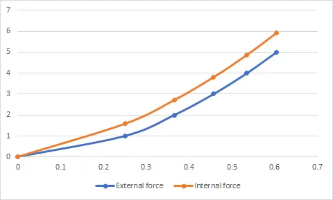
Here, the internal and external forces diverge from equillibrium, which highlights the unsuitability of the explicit method in a static scenario or any scenario where convergence of the solution has a high priority. However, the internal force (f(u)) is shown to be higher than the applied external force, which is not an accurate simulation of a real life scenario.

Implicit analysis: - The displacement, internal & external force are listed below.

Displacement (u)	External force (F(u))	Internal force (f(u))
0	0	0
0.177661	1	1.00032
0.296504	2	2.003318
0.391107	3	3.000931
0.472164	4	4.000364
0.543984	5	5.000181

The resultant plot is shown below.

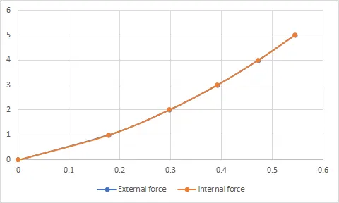
The internal and external forces are almost the same, as shown in the plot. The correction factors assures convergence, which signifies equillibrium of internal & external forces in this scenario. However, the number of calculations required is far greater than that in explicit analysis. The number of calculations required is not consistent in the implicit method either. These factors show that the implicit analysis is well suited for static/quasi-static scenarios but far too computationally demanding for dynamic scenarios.

Conclusion: The explicit and implicit numerical methods are demonstrated for the given function. It shows how these methods alter the dependent variable (displacement or u) in order to get an accurate solution. The advantages and disadvantages for both the methods are also displayed prominently, giving context to their applications.