Week - 2 - Explicit and Implicit Analysis

Consider the case of a simple bar in tension. Suppose that the force in the bar is a nonlinear function of the displacement.

Given the Equation

f(u)= u^3+9*u^2+4*u

Therefore the stifness is

k(u)= df/du = 3*u^2+18*u+4

Explicit Analysis :

Here we are using incremental explict load control scheme. for this example three equal load increments (or steps) of δF=1 unit each are used. The variables used are u for displacement, f for internal force in the bar, F for external force applied on the bar and k for stiffness. Incrmental displacements or incrmental externally applied forces are represented by δu or δF respectively. Use is made of the relationship δF = k*δu. And the analysis goes as follows

Step 1:

 u0 = 0 => k(u0) = 4 , δF = 1
 δu1 = δF/f(u0) = 1/4 = 0.25
 u1 = u0 + δu1 = 0 + 0.25 = 0.25
 

Step 2 :

 K(u1) = 3*(0.25)^2+18*0.25+4 = 8.6875
 δu2 = δF/k(u1) = 1/8.6875 = 0.11511
 u2 = u1 + δu2 = 0.25 + 0.1151 = 0.3651

Step 3 :

 K(u2) = 3*(0.3651)^2+18*(0.3651)+4 = 10.9717
 δF = 1
 δu3 = δF/K(u2)= 1/10.9717 = 0.09114
 u3 = u2 + δu3 = 0.3651 + 0.09114 = 0.45624 

Finally, from the three steps the following results are obtained

F(external) = δF + δF + δF = 3.0

f(internal) = u^3+9*u^2+4*u = 0.4526^3+9*(0.4564)^2+4*(0.45624) 
                            = 0.09497 + 1.8734 + 1.82496
                            = 3.7933

From the above we cane see that external and internal forces are not equilibrium and the following table summerizes the main results of explicit analysis

Table : Summary of Explicit analysis results

Step i	δF(i)	δu(i)	u(i)	F ext (i)	f int (i)	R = f int - F ext
1	1	0.25	0.25	1	1.57812	0.57812
2	1	0.11511	0.3651	2	2.70575	0.70575
3	1	0.09114	0.45624	3	3.7933	0.7933

Implicit Analysis

An implicit analysis is the same as the explicit analysis , except thta at the end of each step Newton - Raphson iterations are used to enforce equilbrium before moving to the next step. here correction must be made to the displacement. this is accamplished by using newton - raphson iterations to minimize the residual R(u) = f int - F ext. from the taylor series and by neglecting the higher order terms we have

 δu(j+1) = -[K(uj)]^(-1)*Rj

Notice that the iteration variable is j and it may take sevral iterations for the norm of the residual. ||R||, to be reduced below thw chosen tolerance criteria.

For the given problem the chosen tolerance is 0.001. and the implicit analysis goes as follows

Step 1

u(0)= 0 => K(u0) = 4 , δF = 1 ,
δu1 = δF/K(u0)= 1/4 = 0.25
u1 = u0 + δu1 = 0.25 
Checking the residue F(ext) = δF = 1
                     f(int) = u1^3+9*u1^2+4*u1 = 1.578125
Therefore residual R(0) = f(int) - F(ext) = 0.578125 > 0.001

So newton Raphson iteration is necessary
Calculate the new total correction to U1 = U1(0)
 δU1 = -[K(U1(0))]^-1*R(0) = -0.115108*0.578125 = -0.066547
u1(1) = u1(0) + δu1 = 0.25-0.066547 = 0.183453 

Check the residual again , F(ext) = 1 
                           f(int) = 0.183453^3+9*0.183453^2+4*0.183453
                                  = 1.042881
Therfore R(1) = 0.042881 > 0.001

Another Iteration is necessary
Calculate the correct u1 = u1(0)
δu(1) = δu(1) - [Ku1(1)]^-1*R(1) 
      = -0.066547 - (0.13507)(0.042881)
      = -0.0723393

Update the value = u1(0) + δu2 = 0.25 - 0.0123393
                               = 0.177660

Check the residula again , F(ext) = δF = 1
                           f(int) = 0.17766^3+9*0.17766^2+4*0.17766
                                  = 1.000377
Residual R(2) = 0.000377 < 0.001

Therfore  u1 = u1(1) = 0.17766 

Step 2:

u(1)= 0.17766 => K(u1) = 7.292569 , δF = 1 ,
δu2 = δF/K(u1)= 1/7.299569 = 0.13713
u2 = u1 + δu2 = 0.17766+0.13713 = 0.31479
 
Checking the residue F(ext) = δF = 1
                     f(int) = u2^3+9*u2^2+4*u2 = 2.182187
Therefore residual R(0) = f(int) - F(ext) = 0.182187 > 0.001

So newton Raphson iteration is necessary
Calculate the new total correction to U2 = U2(0)
 δU1 = -[K(U2(0))]^-1*R(0) = -0.100366*0.182187 = -0.018285
u2(1) = u2(0) + δu1 = 0.3479-0.018285 = 0.296505 

Check the residual again , F(ext) = 1 
                           f(int) = 0.296505^3+9*0.296505^2+4*0.296505
                                  = 2.003324
Therfore R(1) = 0.003324 > 0.001

Another Iteration is necessary
Calculate the correct u2 = u2(0)
δu(2) = δu(1) - [Ku2(1)]^-1*R(1) 
      = -0.018285 - (0.104157)(0.003324)
      = -0.0186312

Update the value = u2(0) + δu2 = 0.31479 - 0.0186312
                               = 0.296159

Check the residula again , F(ext) = δF = 2
                           f(int) = 0.296159^3+9*0.296519^2+4*0.296519
                                  = 2.000003
Residual R(2) = 0.000003 < 0.001

Therfore  u2 = u2(2) = 0.296159 

Step 3:

u(2)= 0.296159 => K(u2) = 9.593992 , δF = 1 ,
δu3 = δF/K(u2)= 1/9.593992 = 0.104231
u3 = u2 + δu3 = 0.296159+0.104231 = 0.400391
 
Checking the residue F(ext) = δF = 3
                     f(int) = u3^3+9*u3^2+4*u3 = 3.108568
Therefore residual R(0) = f(int) - F(ext) = 0.108568 > 0.001

So newton Raphson iteration is necessary
Calculate the new total correction to U3 = U3(0)
 δU1 = -[K(U3(0))]^-1*R(0) = -0.085558*0.108508 = -0.009284
u2(1) = u2(0) + δu1 = 0.400391-0.009284 = 0.391107 

Check the residual again , F(ext) = 3 
                           f(int) = 0.391107^3+9*0.391107^2+4*0.391107
                                  = 3.00093556
Therfore R(1) = 0.00093556 > 0.001

No further iteration required  

The results of the implicit analysis are summerized in the below table. It is evident from the table that the external forces and internal forces are coming into equlibrium

Step i	δFi	ui	F(ext)i	f(int)i	Residual (R)
1	1	0.177660	1	1.000377	0.000377
2	1	0.296159	2	2000003	0.000003
3	1	0.391107	3	3.000935	0.000935

Plot of the results :

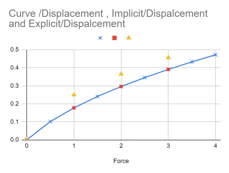
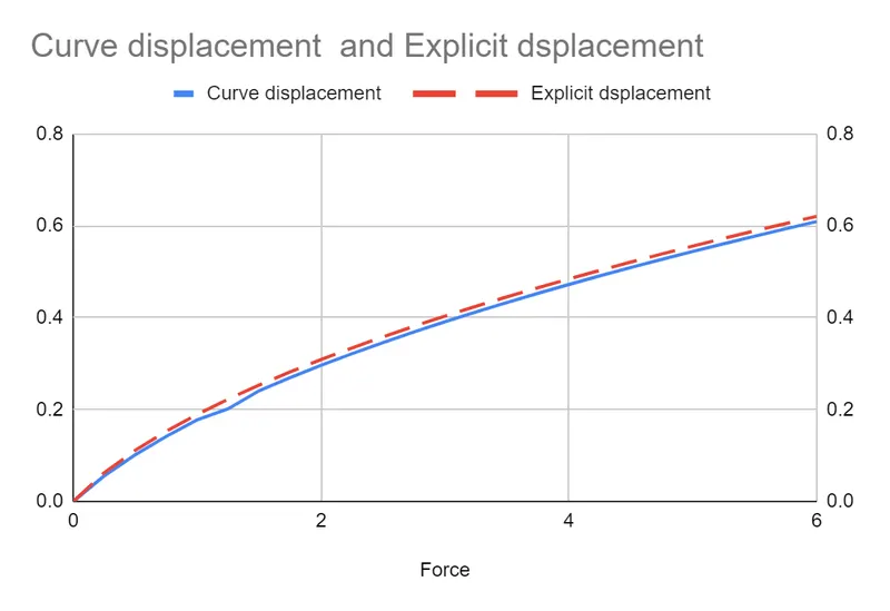
A plot of the results are shown in the below graphs a. it is evident from the plot that the explicit analysis drifts from the exact solution. If 20 increments are used the explicit anallysis more closley follows the exact solution as shown in the graph b. However, even with more incrments the explicit analysis still drifts from the exact solution. The drift from the exact solution illusrates that lack of equilibrium between the internal and external forces. To correct this problem an implicit analysis is required. The results of the implict analysis are shown in the graph a. The Newton Raphson iterations correct the incremental steps so that they land on the exact solution according to the specified tolerance. Excellent agreement is acheived with just 3 incrments and in each step only two newton-Raphson iterations are required.

Graph a (displacement vs force) of orginal curve , implicit & explicit curves

Blue - actual curve

red - implicit

yellow - explicit

graph b (displacemnt vs force) for actual & explicit (20 increments)

Blue - actual curve

red - explicit curve

Discussion :

The above discuused case is the simple one. there are very complex strucutres are available with may degrees of freedom and it requires a more sophisticated convergence criteria.

• Note that an exact expression for force vs displacement is not always known
• More discussion later such as which is better implicit or explicit ?
• When to use explicit instead oif implicit?
• how does this example relate to the nonlinear strucutre problem with many degrees of freedom?
• what increment should be used in explicit?
• what incrment size should be used in implicit ?
• Increment size may affect convergence rate. If the incrment size is appropriate the Newton Raphson iterations converge quadratically.
• Many things to see later

Conclusion

A non linear analysis is illustarted using an incrmental explicit and implicit procedure. and the results ar set for comparison. it is evident from the results that the explicit analysis drifts from the true solution. And the implict is almost equlibrium with the external and internal forces.

Above used technique uses the load control scheme. there are other schemes such as displacement control, arc length control and genralized displacement control. and can be refered the books

References

• Nonlinear static - Explicit and implicit analysis Example by Louie L. yaw, Wallla walla university, draft date may 27, 2009