Week - 2 - Explicit and Implicit Analysis
AIM: To perform a Cubic partial differential Equation to solve Both explicit and implicit methods with a tolerance of 0.001 with proper notes of Implicit and Explicit.
Methods used to perform in Solver in the FEA domain:
To solve the equation we can use Implicit and explicit methods:
What are Explicit methods:
The explicit analysis offers a faster solution in events where there is a dynamic equilibrium or otherwise:
Sum of all forces = mass x acceleration
The explicit method should be used when the strain rates/velocity is over 10 units/second or 10 m/s respectively. These events can be best exampled by extreme scenarios such as an automotive crash, ballistic event, or even meteor impact. In these cases, the material models do not only need to account for the variation of stress with strain but also the strain rate. On this scale, the strain rates play a particularly important contribution.
No iterations are required because nodal accelerations are calculated directly. We are taking the kinematic conditions from one small increment of time and using them to calculate those conditions at the next. Hence, the state at the end of the increment in question is based only upon the displacements, velocities, and accelerations at the beginning of that same increment. What has gone previously is irrelevant and convergence is a non-issue.
What are Implicit methods:
The implicit method should be used when the events are much slower and the effects of strain rates are minimal. Once the growth of stress as a function of strain can be established, these can be analyzed using implicit methods. In this case, one can consider a static equilibrium such that:
Sum of all forces = 0
This covers many of the most common engineering problems.
In layman’s terms, implicit analysis works by trying solutions or iterations in attempts to establish static equilibrium (within a certain tolerance) with respect to the loading or displacement applied. We are solving for unknown displacements through matrix inversion. When the problem is nonlinear in any way – think geometry, material, contact – the solution is obtained over a number of small increments and the solution for the current increment is based upon the result from the previous one (and so on). When we have large models or significant nonlinearity, inverting the matrix is highly computationally expensive and sometimes impossible. When solutions can be found, they are unconditionally stable and allow reasonably large chunks of ‘time’ (although it’s more like chunks of displacement) to be solved for at once.
Use Implicit when:
-
Sum of forces = 0 (all the way through the analysis)
-
Strain rates are very low (<10^-3 per second)
-
Velocity is irrelevant
-
An increase in stress can be defined easily as a function of strain only
Examples: static forces, slowly applied displacements, self-weight, constant pressure loading.
Use Explicit when:
-
Sum of forces = mass x acceleration
-
Strain rates are above 10^-3 per second
-
Velocity is above 10m per second
-
An increase in stress is a function of both strain and strain rate
Examples: automotive crashes, ballistic events, and metal stamping.
where u= displacement , f= internal force in bar, F= external force in bar
∆u = incremental displacements, ∆F = incremental external applied forces.
using relation, ∆F = k∆u,
Step1 :
Take, u0 = 0.0, apply in (2)
(2) => k(u0)= 3x0^2+18x0+4 = 4
now, ∆u1 = ∆F/k(u0) = 1/4 = 0.25
u1 = u0+∆u1= 0.25
u1 = 0.25;
Step 2 :
Take u1= 0.25
(2) => k(u1)= 3x0.25^2+18x0.25+4 = 8.6875
now, ∆u1 = ∆F/k(u1) = 1/8.6875 = 0.1151
u2 = u1+∆u2= 0.3651
u2 = 0.3651;
Step 3 :
Take u2= 0.3651
(2) => k(u2)= 3x0.3651^2+18x0.3651+4 = 10.9716
now, ∆u2 = ∆F/k(u2) = 1/10.9716 = 0.09114
u3 = u2+∆u3= 0.46
u3 = 0.46;
Finally, To determine whether the analysis is in equilibrium,
F(ext) = ∆F+∆F+∆F = 3
f(int) = (1) => (0.46)^3+(9x0.46^2)+(4x0.46) = 3.841
F(ext) ≠ f(int), so they are not in equilibrium.
Result of Explicit methods:
| Explicit method | ||||||
| Step i | ∆Fi | ∆ui | ui | F | F(u) | F(u) - F = R(0) |
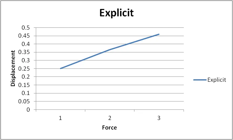
| 1 | 1 | 0.25 | 0.25 | 1 | 1.578 | 0.578 |
| 2 | 1 | 0.1151 | 0.3651 | 2 | 2.708 | 0.708 |
| 3 | 1 | 0.09114 | 0.46 | 3 | 3.841 | 0.841 |
Graph of Explicit method Force vs Displacement:
Solving using Implicit Method:
where u= displacement , f= internal force in bar, F= external force in bar
∆u = incremental displacements, ∆F = incremental external applied forces.
using relation, ∆F = k∆u
Checking for Newton's Rasphson Method:
Take, u0 = 0.0, apply in (2)
(2) => k(u0)= 3x0^2+18x0+4 = 4
now, ∆u1 = ∆F/k(u0) = 1/4 = 0.25
u1 = u0+∆u1= 0.25
`delta`F1 = 1;
| Implicit Method | ||||||
| Step i | ∆Fi | ∆ui | ui | F | F(u) | F(u) - F = R(0) |
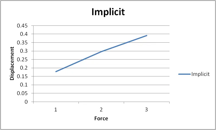
| 1 | 1 | 0.25 | 0.178 | 1 | 1.043 | 0.043 |
| 2 | 1 | 0.3152 | 0.297 | 2 | 2.008 | 0.008 |
| 3 | 1 | 0.401 | 0.3911 | 3 | 3.00085 | 0.00085 |
Graph of Implicit method Force vs Displacement:
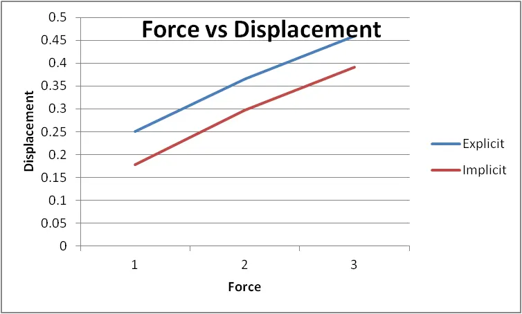
The Implicit and Explicit numerical analysis is carried out for given equation.
From the graph, Implicit method is more accurate but time consuming and solemnly depends on element size and timestep whereas explicit deviates slightly from exact result and needs more iterations to obtain good result.