Week - 2 - Explicit and Implicit Analysis

Consider a problem as shown below solve it using Both Explicit and Implicit Method and compare it with Exact solution.

F(u)=u³+9u²+4u

Explicit Analysis:

Given: F(u)=u³+9u²+4u

Stiffness of the bar is df/du=k(u)=3u²+18u+4

However, if the nonlinear force versus displacement relationship is not known, but the stiffness is known, it is possible to construct the graph of force versus displacement numerically. One method is to use an incremental explicit load control scheme.

The variables used are u for displacement, f for internal force in the bar, F for external force applied to the bar and k for stiffness. Incremental displacements or incremental externally applied forces are represented as Δu or ΔF, respectively. Use is made of the relationship ΔF = k Δu.

Rearrange the above formula, We get Δu = ΔF/k

Step 1:

u0 = 0, ⇒ k(u0) = 4, ΔF = 1, Δu1 = ΔF/k(u0) = 1/4 = 0.25,

u1 = u0 + Δu1 = 0+0.25=0.25

Hence u₁₌0.25

f_ext =1

f_int = (0.25)³+9(0.25)²+4(0.25) =1.579

Step 2:

u₁₌0.25⇒ k(u1) = 3(0.25)² + 18(0.25)+4 = 8.69, ΔF = 1, Δu2 = ΔF/k(u1) = 1/8.69 =0.115

u2 = u1 + Δu2 = 0.25+0.115 =0.365

Hence u₂=0.365

f_ext =1

f_int = (0.365)³+9(0.365)²+4(0.365) =2.708

Step 3:

u₂=0.365⇒ k(u2) = 3(0.365)²+18(0.365)+4 = 10.72,ΔF = 1, Δu3 = ΔF/k(u2) = 1/10.72 =0.093, u3 = u2+Δu3 =0.365+0.093 =0.458

Hence u₃=0.458

f_ext =1

f_int = (0.458)³+9(0.458)²+4(0.458) =3.808

Finally, from the three steps the following results are obtained.

Fext = ΔF + ΔF + ΔF = 3.0

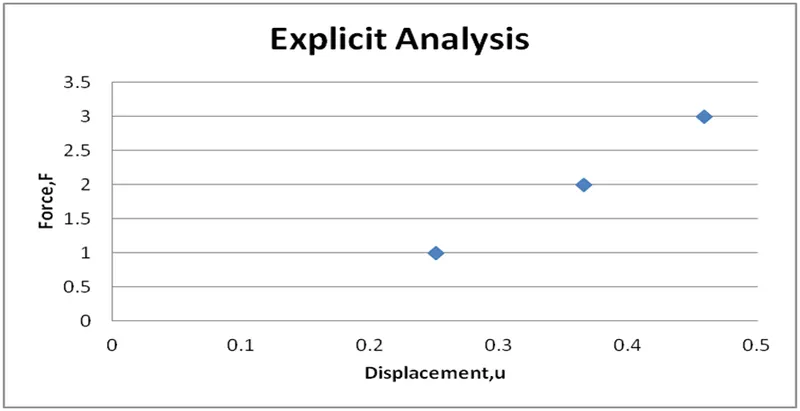
Summary of Explicit Analysis Results

Step i	ΔFi	Δui	ui	(Fext)i	(fint)i	fint − Fext = R
1	1	0.25	0.25	1	1.579	0.579
2	1	0.115	0.365	2	2.708	0.708
3	1	0.093	0.458	3	3.808	0.808

Implicit analysis

An implicit analysis is the same as the explicit analysis, except that at the end of each step Newton-Raphson iterations are used to enforce equilibrium before moving to the next step.

Basically, an incremental force is applied to advance the solution forward at the beginning

of a step. However, internal forces and external forces will not be in equilibrium unless the

stiffness is linear for the given step. Hence, in order to achieve equilibrium, corrections must

be made to the displacement. This is accomplished by using Newton-Raphson iterations to

minimize the residual, R(u) = fint − Fext.

δ u^j+1 = −[k(u^j)]⁻¹R_j .

Given: F(u)=u³+9u²+4u

Stiffness of the bar is df/du=k(u)=3u²+18u+4

Step 1 :

u₀=0 ⇒k(u₀ ) = 3(0)² + 18(0) + 4 = 4, ΔF = 1, Δu1 = ΔF/k(u0) = 1/4 = 0.25,

u1 = u0 + Δu1 = 0+0.25=0.25

Hence u₁₌0.25

Check for Residual; f_ext =1; f_int = (0.25)³+9(0.25)²+4(0.25) =1.579;

R = f_int - f_ext=1.578 – 1 =0.578

R(0) >0.01 Hence Newton-Raphson iterations are necessary.

Iteration 1:

Calculating the new total correction to u_{1 =} u₁⁽⁰⁾

δ u ⁽¹⁾= −[k(u₁⁰ )] ^-1. R = - (8.6875) (0.578) = - 0.0665

Where, K(u₁⁰ ) = 3(0.25)²+18(0.25)+4 = 8.6875

Therefore update value of u is, u₁⁽¹⁾ = u₁⁰ + δ u⁽¹⁾ = 0.25 - 0.0665 ;u = 0.1834

Check the residual again; f_ext =1; f_int = (0.1834)³+9(0.1834)²+4(0.1834) =1.0432;

R = f_int - f_ext=1.0432 – 1 =0.0432 >0.01; Hence Newton-Raphson iterations are necessary

Iteration 2:

Calculating the new total correction to u_{1 =} u₁⁽¹⁾

δ u ⁽²⁾= δ u 1−[k(u₁¹ )] ^-1. R =- 0.0665 - (7.402) (0.0432) = - 0.0723

Where, K(u₁¹ ) = 3(0.1834)²+18(0.1834)+4 = 7.402

Therefore update value of u is, u₁⁽²⁾ = u₁⁰ + δ u⁽²⁾ = 0.25 - 0.0723 ;u₁= 0.1776

Check the residual again; f_ext =1; f_int = (0.1776)³+9(0.1776)²+4(0.1776) =1.0006;

R = f_int - f_ext=1.0006 – 1 =0.0006 <0.01:

Hence Newton-Raphson iterations are not necessary

Step 2 :

u₁= 0.1776

u₁=0.1776 ⇒k(u₀ ) = 3(0.1776)² + 18(0.1776) + 4 = 7.291, ΔF = 1, Δu1 = ΔF/k(u0) = 1/7.291 = 0.137,

u2 = u1 + Δu2 = 0.1776+0.137=0.3147

Hence u₂₌0.3147

Check for Residual; f_ext =2; f_int = (0.3147)³+9(0.3147)²+4(0.3147) =2.181;

R = f_int - f_ext=2.181 – 2 =0.181

R(0) >0.01 Hence Newton-Raphson iterations are necessary.

Iteration 1:

Calculating the new total correction to u_{2 =} u₂⁽⁰⁾

δ u ⁽¹⁾= −[k(u₂⁰ )] ^-1. R = - (9.9617)^-1 (0.181) = - 0.0182

Where, K(u₁⁰ ) = 3(0.3147)²+18(0.3147)+4 = 9.9617

Therefore update value of u is, u₁⁽¹⁾ = u₁⁰ + δ u⁽¹⁾ = 0.3147 - 0.0182;u₂ = 0.2962

Check the residual again; f_ext =2; f_int = (0.2962)³+9(0.2962)²+4(0.2962) =2.00039;

R = f_int - f_ext=2.00039 – 2 =0.00039 <0.01; Hence Newton-Raphson iterations are not necessary

Step 3 :

U₂= 0.2962

U₂=0.2962 ⇒k(u₁ ) = 3(0.2962)² + 18(0.2962) + 4 = 9.6007, ΔF = 1, Δu1 = ΔF/k(u0) = 1/9.6007 = 0.1041,

U3 = u2+ Δu3= 0.2962+0.1041=0.4006

Hence u₃₌0.4006

Check for Residual; f_ext =3; f_int = (0.4006)³+9(0.4006)²+4(0.4006) =3.116;

R = f_int - f_ext=3.116 – 3 =0.116

R(0) >0.01 Hence Newton-Raphson iterations are necessary.

Iteration 1:

Calculating the new total correction to u_{3 =} u₃⁽⁰⁾

δ u ⁽¹⁾= −[k(u₃⁰ )] ^-1. R = - (11.683)^-1 (0.116) = - 0.0092

Where, K(u₁⁰ ) = 3(0.4006)²+18(0.4006)+4 = 11.683

Therefore update value of u is, u₃⁽¹⁾ = u₃⁰ + δ u⁽¹⁾ = 0.4006- 0.0092;u₃ = 0.3911

Check the residual again; f_ext =3; f_int = (0.3911)³+9(0.3911)²+4(0.3911) =3.0008;

R = f_int - f_ext=3.0008 – 3 =0.0008 <0.01; Hence Newton-Raphson iterations are not necessary

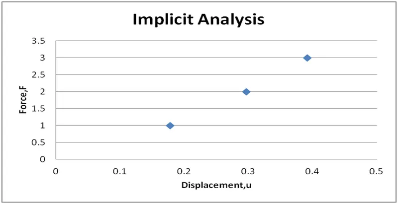
Summary of Implicit Analysis Results

Step i	ΔFi	Δui	ui	(Fext)i	(fint)i	fint − Fext = R
1	1	0.25	0.1776	1	1.0006	0.0006
2	1	0.137	0.2962	2	2.00039	0.0003
3	1	0.1041	0.3911	3	3.0008	0.0008

Exact Result:-Using Calculator

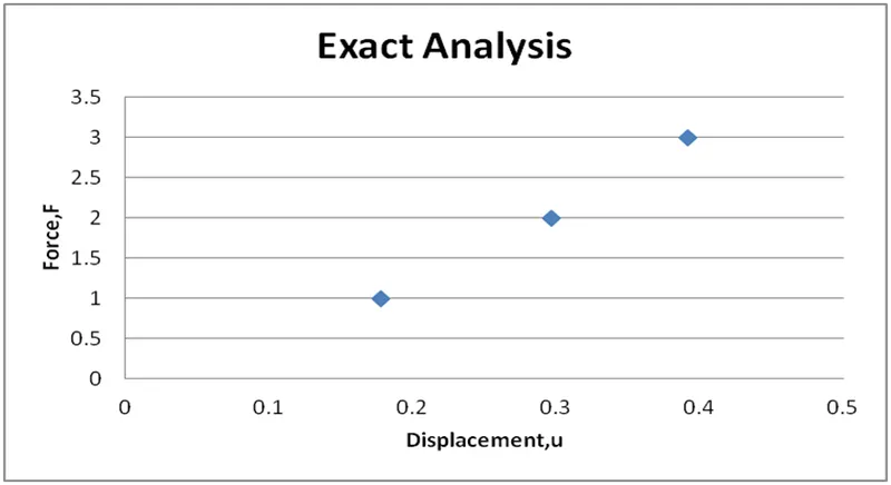
THIRD ORDER POLYNOMIAL OF NON LINEAR DISPLACEMENT EQUATION

Take F(u)= u³+9u²+4u ;

u³+9u²+4u -F(u) = 0

F(u₁) = 1 ; u³+9u²+4u -1 = 0 equation is solved by using scientific calculator with polynomial degree 3 and the value of u₁ =0.1176

F(u₂ ) = 2 ; u³+9u²+4u -2 = 0 this equation is solved by using scientific calculator with polynomial degree 3 and the value of u₂ =0.2961

F(u₃ ) = 3 ; u³+9u²+4u -3= 0 this equation is solved by using scientific calculator with polynomial degree 3 and the value of u₃ =0.3910

Step i	ui
1	0.1776
2	0.2961
3	0.3910

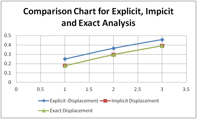
Comparison Table of Explicit, Implicit and Impact analysis for Force vs Displacement

Force	Explicit -Displacement	Implicit Displacement	Exact Displacement
1	0.25	0.1776	0.1775
2	0.365	0.2962	0.2961
3	0.458	0.3911	0.391

Conclusion :

1.It is evident that for the given polynomial equation among the three methods like Explicit analysis, Implicit analysis and Exact analysis, Implicit analysis results matches with Exact analysis as shown in above figure.

2.This is due to Newton raphson method because it reduces the residues in implicit analysis where as explicit analysis have no such iterations.

3.But Implicit analysis which is not suitable for Non linear transient dynamic problem because the curve extends still linear where in that case which is not in real time scenario at that time explicit analyis play a vital role.

Examples:

Implicit analysis Softwares - Abaqus -Strength and durability

Explicit analysis Softwares - Ls Dyna - Crashworthyness Behaviour