Week - 2 - Explicit and Implicit Analysis
F(u) = u3+9u2+4u
EXPLICIT ANALYSIS: In explicit mostly dynamic analysis, nodal accelerations are solved directly (not iteratively) as the inverse of the diagonal mass
matrix times the net nodal force vector where net nodal force includes contributions from exterior sources (body forces, applied
pressure, contact, etc.), element stress, damping, bulk viscosity, and hourglass control. Once accelerations are known at time n,
velocities are calculated at time n+1/2, and displacements at time n+1. From displacements comes strain. From strain comes stress
and the cycle is repeated.
Explicit analysis handles nonlinearities with relative ease as compared to implicit analysis. This would include the treatment of contact
and material nonlinearities. With this method is that you do need many small increments for good accuracy and it is time-consuming.
where u= displacement , f= internal force in bar, F= external force in bar
∆u = incremental displacements, ∆F = incremental external applied forces.
using relation, ∆F = k∆u,
IMPLICIT ANALYSIS :
Implicit analysis requires a numerical solver to invert the stiffness matrix once or even several times over the course of a load/time step. This matrix inversion is an expensive operation, especially for large models. It is mostly used for static analysis. Implicit uses Newton-Raphson iterations to enforce equilibrium. If done correctly, the Newton-Raphson iterations will have a very desirable quadratic convergence rate.
Implicit transient analysis has no inherent limit on the size of the time step. As such, implicit time steps are generally several
orders of magnitude larger than explicit time steps.
where u= displacement , f= internal force in bar, F= external force in bar
∆u = incremental displacements, ∆F = incremental external applied forces.
using relation, ∆F = k∆u, Tolerance= 10^-2
Step1 :
Take, u0 = 0.0, apply in (2)
(2) => k(u0)= 3x0^2+18x0+4 = 4
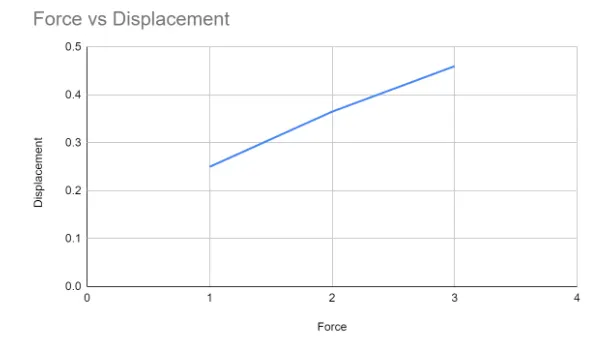
now, ∆u1 = ∆F/k(u0) = 1/4 = 0.25
u1 = u0+∆u1= 0.25
Step 2 :
Take u1= 0.25
(2) => k(u1)= 3x0.25^2+18x0.25+4 = 8.6875
now, ∆u1 = ∆F/k(u1) = 1/8.6875 = 0.1151
u2 = u1+∆u2= 0.3651
Step 3 :
Take u2= 0.3651
(2) => k(u2)= 3x0.3651^2+18x0.3651+4 = 10.9716
now, ∆u2 = ∆F/k(u2) = 1/10.9716 = 0.09114
u3 = u2+∆u3= 0.46
Finally, To determine wheather the analysis is in equlibrium,
F(ext) = ∆F+∆F+∆F = 3
f(int) = (1) => (0.46)^3+(9x0.46^2)+(4x0.46) = 3.841
F(ext) ≠ f(int), so they are not in equilibrium.
IMPLICIT :
Step 1:
Take u0=0,
(2) => k(u0) =3(0)^2+18x0+4 = 4
now, ∆u1 = ∆F/k(u0) = 1/4 = 0.25
u1 = u0+∆u1= 0.25
Checking residual, R
F(ext)=∆F=1 f(int)=(1)=> (0.25)^3+(9x(0.25)^2)+(4x0.25) =1.578
R0 = 1.578-1 = 0.578 > 10^-2
so, Newton-Raphson iterations are necessary.
calc. the correction to u1=u1(0)
wkt, ẟu(1) = -[k(u1(0)]^-1 x R0 = -[(3x0.25^2)+(18x0.25)+4]^-1 x 0.578 = -0.0665
updated, u1(1) = u1(0)+ẟu(1) = 0.25-0.0665 = 0.1835
Check residual again, R1,
F(ext)= 1, f(int) = (0.1835)^3+(9x0.1835)^2+(4x0.1835) = 1.0432
R1 = 1.0432-1 = 0.0432 > 10^-2, another Newton-Raphson iteration needed.
Calc. the correction to u1 = u1(1),
ẟu(2) = ẟu(1)-[k(u1(1)]^-1 x R1 = (-0.0665)-(8.6875)^-1 x(0.0432) = -0.0714
updated, u1(2) = u1(1)+ẟu(2) = 0.25-0.0714 = 0.1786
Checking Residual again,R2,
F(ext)=1, f(int)= (1) => (0.1786)^3+(9x0.1786^2)+(4x0.1786) = 1.0071
R2 = 1.0071-1 = 0.0071 < 10^-2
Therefore no iterations needed, final u1 = 0.1786
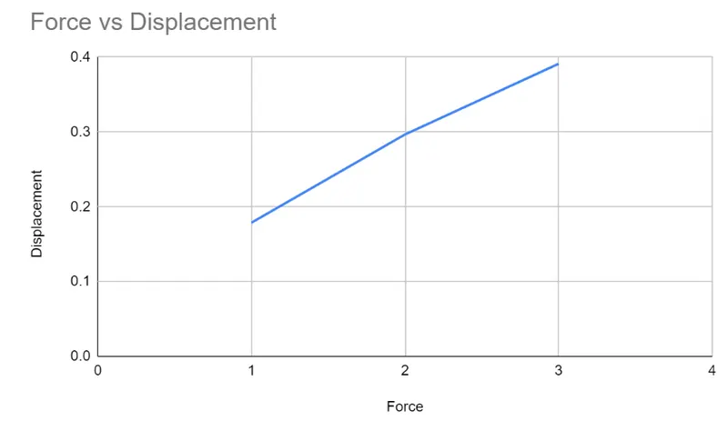
Conclusion: After doing both Implicit and Explicit analysis for the given equation. we found that the implicit solution is accurate and time-consuming, whereas the Explicit is fast but not as accurate as of the Implicit method.