Week - 2 - Explicit and Implicit Analysis

AIM:-

To solve the equation F(u) = u3+9u2+4u in Explicit and implicit methods with tolerance of 0.001.

IMPLICIT METHOD:-

One method of solving for the unknowns {x} is through matrix inversion (or equivalent processes). This is known as an implicit analysis. When the problem is nonlinear, the solution is obtained in a number of steps and the solution for the current step is based on the solution from the previous step. For large models, inverting the matrix is highly expensive and will require advanced iterative solvers (over standard direct solvers). Sometimes, this is also known as the backward Euler integration scheme. These solutions are unconditionally stable and facilitate larger time steps. Despite this advantage, the implicit methods can be extremely time-consuming when solving dynamic and nonlinear problems.

EXPLICIT ANALYSIS:-

Explicit analyses aim to solve for acceleration (or otherwise {x´´}). In most cases, the mass matrix is considered as “lumped” and thus a diagonal matrix. Inversion of a diagonal matrix is straightforward and includes inversion of the terms on the diagonal only. Once the accelerations are calculated at the nth step, the velocity at n+1/2 step and displacement at n+1 step are calculated accordingly. In these calculations, the scheme is not unconditionally stable and thus smaller time steps are required. To be more precise, the time step in an explicit finite element analysis must be less than the courant time step (i.e., the time taken by a sound wave to travel across an element) while implicit analyses have no such limitations.

Difference between Implicit and Explicit methods.

IMPLICIT	EXPLICT
It deals static and dynamic problems	It deals dynamic and shock problems
it is always stable	It is conditional stability
It is global resolution i.e need of convergence	It is element by element calculation
It is too expensive	It is less expensive
Time step is very large	Time step is very low
It is low Robustness	It is high Robustness

SOLVING THE EQUATION IN EXPLICIT METHOD:-

F(u) = u^3+9u^2+4u

K(u) = df/du = d/du(u^3+9u^2+4u)

K(u) = 3u^2+18u+4

STEP 1:-

Take u0 = 0,

K(u0) = 3(0)^2+18(0)+4

K(u0) = 4

ΔF1 = 1,

Δu1 = ΔF1/K(u0)

= 1/4

Δu1 = 0.25

u1 = u0+Δu1

= 0+0.25

u1 = 0.25

STEP 2:-

u1 = 0.25

K(u1) = 3(0.25)^2+18(0.25)+4

= 0.1875+4.5+4

K(u1) = 8.6875

ΔF2 = 1,

Δu2 = ΔF2/K(u1)

= 1/8.6875

Δu2 = 0.1151

u2 = u1+Δu2

= 0.25+0.1151

u2 = 0.3651

STEP 3:-

u2 = 0.3651

K(u2) = 3(0.3651)^2+18(0.3651)+4

= 0.4+6.57+4

K(u2) = 10.97

ΔF3 = 1,

Δu3 = ΔF2/K(u1)

= 1/10.97

Δu3=0.0911

u3 = u2+Δu3

= 0.3651+0.0911

u3=0.4562

Finally, from the three steps the following results are obtained.

Fext = ∆F1+ ∆F2+ ∆F3

= 1+1+1

Fext = 3

Fint = (u3)^3+9(u3)^2+4(u3)

= (0.4562)^3+9(0.4562)^2+4(0.4562)

= 0.949+1.873+1.8248

Fint = 3.79

From rthe above results it is clearly evident that the External force and Internal forces are in non-equilibrium.Beacause external force is not equal to the internal force.

Table 1: Summary of explicit analysis results

Steps	ΔF	Δu	u	Fext	Fint	R=Fint-Fext
1	ΔF1=1	Δu1=0.25	u1=0.25	Fext1=1	Fint1=1.57	0.57
2	ΔF2=1	Δu2=0.1151	u2=0.3651	Fext2=2	Fint2=2.7	0.7
3	ΔF3=1	Δu3=0.0911	u3=0.4562	Fext3=3	Fint3=3.79	0.79

SOLVING THE EQUATION IN IMPLICIT METHOD:-

F(u) = u^3+9u^2+4u

K(u) = df/du = d/du(u^3+9u^2+4u)

K(u) = 3u^2+18u+4

ΔF1 = 1,

K(u0) = 3(0)^2+18(0)+4

K(u0) = 4

Δu1 = ΔF1/K(u0)

= 1/4

Δu1 = 0.25

u1 = u0+Δu1

= 0+0.25

u1 = 0.25

Fext1 = ΔF1

Fext1 = 1

Fint1 = F(u1)=(0.25)^3+9(0.25)^2+4(0.25)

Fint1 = 1.578.

Resedual R1 = Fint-Fext

= 1.578-1

R1 =0.578.

R1> 10^−2 ⇒ Newton-Raphson iterations are necessary.

Calculate the corection to u1=u1(0)

δu(1) = −[k(u(0)1)]^−1 *(R1)

= -(8.687)^-1*(0.578)

δu(1) =-0.0665.

updated value of u(1)1 = u(0)1 + δu(1)

= 0.25+(-0.0665)

= 0.1835

Check the resedual again

R2 = Fint - Fext

= 1.04-1

R2 =0.04 so resedual tollerance is not with in the limit, we need one corection factor.

Calculate the corection to u(1)1=u1(1)

δu(2) = −[k(u(1)1)]^−1 *(R2)

= -(7.4)^-1*0.04

δu(1) = -0.0054

updated value of u(2)1= u(1)1 + δu(2)

=0.1835-0.0054

u(2)1=0.1781

Check the resedual again

R3 = Fint - Fext

= 1.003-1

R3 = 0.003 The tolerance is with in limit.

Tabulated Values:

step	u	corrected u	ΔF	Fext	Fint	corrected Fint	R
1	0.25	0.178	1	1	1.57	1	0.57
2	0.37	0.31	1	2	2.70	2	0.7
3	0.456	0.391	1	3	3.79	3	0.79

PLOT OF RESULTS:-

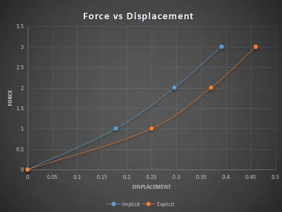
CONCLUSION:-

Thus, both the Implicit and Explicit methods are used to solve the given third-order polynomial problem under a tensile strain.