Week - 2 - Explicit and Implicit Analysis
What do you mean by Implicit and Explicit Analysis?
-We use implicit and explicit solvers to solve any dynamic problems.
-The basic difference between implicit and explicit is that, they differ in the approach to time increments.
-In implicit analysis each time step has to converge and also we can set longer time increments. Where as in explicit no convergence happens at every time increment but, for the solution to be accurate time increments must be super small.
-In general, when we want ot solve a dynamic problem, we are asking the solver to calculate the series of time increments to see what is going on in the model. In each of those increments time slightly increases. This also changes the load in the model. This is why we need to have a time-dependent chart for load. So, the solver will know what load should be applied at which time increment.
-To this extent, it works the same as load increment in static analysis. Also, since we are incrementing time, inertia effects can be taken into account when things are happening fast enough.
-Both impicit and explicit analysis does more or less the same thing. They divide the analysis time into small increments and then analyze what is going on in our model one increment of time after another.
Explicit Analysis:
-The analysis runs in a way such that the analysis does'nt have to converge at every time step. There are no convergence criteria to check and no iterations.
-Instead of verifying the global equilibrium, solver assumes that the equilibrium simply exists. This means that the solver goes straight into calculation of local finite variables. It calculates all of the local finite element variables for given increment and moves to the next one.
-Time increment in explicit analysis is very short. It's the time in which an elastic wave can travle through a single finite element of your model. Of course, this is verified for all finite elements in your model and the smallest time is selected.
Implicit Analysis:
-Implicit analysis works in a way, that in each time increment, the global equilibrium in the model is established. This means that each increment has to converge.
-Since global equilibrium is verified at each time increments, those increments can be large. Each time increment computes slowly since iterations are needed to get to the global equilibrium.
Explicit Analysis:
If the nonlinear force versus displacement relationship is not known, but the stiffness is known, it is possible to construct the graph of force versus displacement numerically.
Step-1:
u0 = 0.0, ⇒ k(u0) = 4, deltaF = 1, deltau1 = F/k(u0) = 0.25, u1 = u0 + u1 = 0.25
Step-2:
k(u1) = 3*(0.25)^2+18*0.25+4=0.1875+4.5+4=8.6875, deltau2 = deltaF/k(u1) = 0.1151, u2 = u1 + u2 = 0.3651
Step-3:
k(u2) = 3*(0.3651)^2+18*0.3651+4 = 10.7178, deltaF = 1, deltau3 = deltaF/k(u2) = 1/10.7178, u3 = u2+deltau3=0.4584
Finally, from the three steps the following results are obtained.
(fint)1= u1^3+9u1^2+4*u1=0.25^3+9*0.25^2+4*0.25=1.5781
(fint)2=u2^3+9u2^2+4*u2=0.3651^3+9*0.3651^2+4*0.3651=2.7087
(fint)3=u3^3+9u3^2+4*u3=0.4584^3+9*0.4584^2+4*0.4584=3.821
Step i Deltafi deltaUi Ui (fext)i (fint)i fint-fext=R
1 1 0.25 0.25 1 1.5781 0.5781
2 1 0.1151 0.3651 2 2.7087 0.7087
3 1 0.0933 0.4584 3 3.821 0.821
Now, from the above results we can say that the external and internal forces are not in equilibrium.
Implicit Analysis:
An implicit analysis is the same as the explicit analysis, except that at the end of each step, iterations are used to enforce equilibrium before moving to the next step. Basically, an incremental force is applied to advance the solution forward at the begining of a step. However, internal forces and external forces will not be in equilibrium unless the stiffness is linear for the given step. Hence, in order to achieve equilibrium, corrections must be made to the displacement.
Step-1:
U0=0, =>K(U0)=4, deltaF=1, deltaU1= deltaF/K(U0)=0.25, U1=U0+deltaU1=0.25
(Fint)1= U1^3+9U1^2+4*U1=0.25^3+9*0.25^2+4*0.25=1.5781
R^0=Fint-Fext=1.5781-1=0.5781
||R^0||>10^-2=>Newton-Raphson Iterations is necessary
The correction is deltaU^1= -[K(U1^0)]^-1*R^0=-[3*0.25^2+18*0.25+4]^-1*0.5781=-0.0665
=>U1^1=U1^0+dU^1=0.25-0.0665=0.1835
(Fint)1=U1^3+9U1^2+4*U1=1.0432>10^2 =>Newton-Raphson Iterations is necessary
The correction is deltaU^2=-[K(U1^1)]^-1*R^1=-[3*0.1835^2+18*0.1835+4]^-1*0.0432=-0.0058
U1^2=U1^0+U1^1+dU^2=0.25-0.0665-0.0058=0.1777
(Fint)1^2=U1^3+9*U1^2+4*U1=0.1777^3+9*0.1777^2+4*0.1777=1.0006
R^2=Fint-Fext=1.0006-1=0.0006<10^-2
So,(Fint)1=1.0006
Step-2:
(Fint)2=U2^3+9U2^2+4*U2=0.3651^3+9*0.3651^2+4*0.3651=2.7087
R^0=Fint-Fext=2.7087-2=0.7087
||R^0||>10^-2 => Newtons-Raphson Iterations are necessary
The correction is deltaU^1=-[K(U2^0)]^-1*R^0=-[3*0.3651^2+18*0.3651+4]^-1*0.5781=-0.0646
U2^1=U2^0+dU^1=0.3651-0.0646=0.3005
(Fint(2^1=U2^3+9*U2^2+4*U2=0.3005^3+9*0.3005^2+4*0.3005=2.037
R^1=Fint-Fext=2.037-2=0.037>10^-2
The correction is deltaU^2=-[K(U2^1]^-1*R^1=-[3*0.3005^2+18*0.3005+4]^-1*0.037=-0.0038
U2^2=U2^0+U2^1+dU^2=0.3651-0.0646-0.0038=0.2967
(Fint)1^2=U1^3+9*U1^2+4*U1=0.2967^3+9*0.2967^2+4*0.2967=2.0052
R^2=Fint-Fext=2.0052-2=0.0052<10^-2
So, (Fint)2=2.0052
Step-3:
(Fint)3=U3^3+9U3^2+4*U3=0.4584^3+9*0.4584^2+4*0.4584=3.821
R^0=Fint-Fext=3.821-3=0.821
||R^0||>10^-2 =>Newton Raphson Iterations are necessary
The correction is deltaU^1=-[K(U3^0)]^-1*R^0=-[3*0.4584^2+18*0.4584+4]^-1*0.821=-0.0637
U3^1=U3^0+dU^1=0.4584-0.0637=0.3947
(Fint)3^1=U3^3+9*U3^2+4*U3=0.3947^3+9*0.3947^2+4*0.03947=3.0424
R^1=Fint-Fext=3.0424-3=0.0424>10^-2
The correction is deltaU^2=-[K(U3^1)]^-1*R^1=-[3*0.3947^2+18*0.3947+4]^-1*0.0424=-0.0037
U2^2=U2^0+U2^1+dU^2=0.4584-0.0637-0.0037=0.3911
(Fint)1^2=U1^3+9U1^2+4*U1=0.3911^3+9*0.3911^2+4*0.3911=3.0009
R^3=Fint-Fext=3.0009-3=0.0009<10^-2
So, (Fint)3=3.0009
Step i Deltafi Ui (fext)i (fint)i fint-fext=R
1 1 0.1777 1 1.0006 0.0006
2 1 0.2967 2 2.0052 0.0052
3 1 0.3911 3 3.0009 0.0009
Graphs:
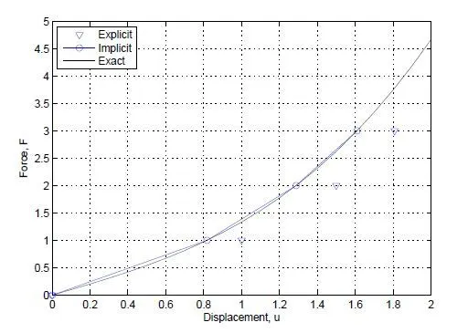
From this graph we can see that even with more increments the explicit analysis still drifts from the exact solution. The drift from the exact solution illustrates the lack of equilibrium between the internal and external forces. To correct for this problem an implicit analysis is required. The results for the implicit analysis aa per this graph. The Newton-Raphson iterations correct the incremental steps so that they land on the exact solution according to the specified tolerance. Excellent agreement is achieved with just 3 increments and in each step only two Newton-Raphson iterations are required.
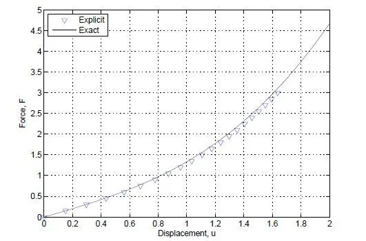
It is evident from the plot that the explicit analysis drifts from the exact solution. If 20 increments are used the explicit analysis more closely follows the exact solution as shown in in this graph. However, even with more increments the explicit analysis still drifts from the exact solution. The drift from the exact solution illustrates the lack of equilibrium between the internal and external forces. To correct for this problem an implicit analysis is required. A shown in the first graph.
Conclusion:
-The implicit analysis allows you to select how big the time increment should be. This increment will take some time to compute since it has to iterate for global equilibrium first.
-Explicit time increment calculate really fast because they do not iterate for global equilibrium, but the time increment there is not the user's choice.
-The speed of computing is exactly the difference between implicit and explicit. Of course, the size of explicit step depends on our model and computing time depends on the system hardware.